CustomSource#
The CustomSource class was implemented to offer easy integration of user field implementations into Magpylibs object-oriented interface.
Note
Obviously, any field implementation can be integrated. Specifically, fields where superposition holds and interactions do not disturb the sources (e.g. electric, gravitational, …) can benefit from Magpylibs position and orientation interface.
Magnetic Monopole#
In this example we create a class that represents the elusive magnetic monopole, which would have a magnetic field like this
Here the monopole lies in the origin of the local coordinates, \(Q_m\) is the monopole charge and \({\bf r}\) is the observer position.
We create this field as a Python function and hand it over to a CustomSource field_func argument. The field_func input must be a callable with two positional arguments field (can be 'B' or 'H') and observers (must accept ndarrays of shape (n,3)), and return the respective fields in units of mT and kA/m in the same shape.
import numpy as np
import magpylib as magpy

# Create monopole field
def mono_field(field, observers):
    """
    Monopole field

    field: string, "B" or "H
        return B or H-field

    observers: array_like of shape (n,3)
        Observer positions

    Returns: np.ndarray, shape (n,3)
        Magnetic monopole field
    """
    if field=="B":
        Qm = 1          # unit mT
    else:
        Qm = 10/4/np.pi # unit kA/m
    obs = np.array(observers).T
    field = Qm * obs / np.linalg.norm(obs, axis=0)**3
    return field.T

# Create CustomSource with monopole field
mono = magpy.misc.CustomSource(
    field_func=mono_field
)

# Compute field
print(mono.getB((1,0,0)))
print(mono.getH((1,0,0)))
[1. 0. 0.]
[0.79577472 0.         0.        ]
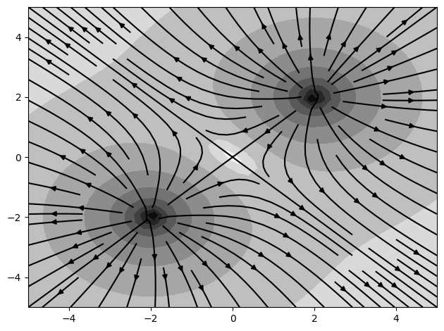
Multiple of these sources can now be combined, making use of the Magpylib position/orientation interface.
import matplotlib.pyplot as plt

# Create two monopole charges
mono1 = magpy.misc.CustomSource(
    field_func=mono_field,
    position=(2,2,0)
)
mono2 = magpy.misc.CustomSource(
    field_func=mono_field,
    position=(-2,-2,0)
)

# Compute field on observer-grid
X, Y = np.mgrid[-5:5:40j, -5:5:40j].transpose((0, 2, 1))
grid = np.stack([X, Y, np.zeros((40, 40))], axis=2)
B = magpy.getB([mono1, mono2], grid, sumup=True)
normB = np.linalg.norm(B, axis=2)

# Plot field in x-y symmetry plane
cp = plt.contourf(X, Y, np.log10(normB), cmap='gray_r', levels=10)
plt.streamplot(X, Y, B[:, :, 0], B[:, :, 1], color='k', density=1)

plt.tight_layout()
plt.show()
Adding a 3D model#
While the CustomSource is graphically represented by a simple marker by default, we can easily add a 3D model as described in Custom 3D models.
# Load Sphere model
trace_pole = magpy.graphics.model3d.make_Ellipsoid(
    dimension=(.3,.3,.3),
    )

for mono in [mono1, mono2]:
    # Turn off default model
    mono.style.model3d.showdefault=False

    # Add sphere model
    mono.style.model3d.add_trace(trace_pole)

# Display models
magpy.show(mono1, mono2)
Subclassing CustomSource#
In the above example it would be nice to make the CustomSource dynamic, so that it would have a property charge that can be changed at will, rather than having to redefine the field_func and initialize a new object every time. In the following example we show how to sub-class CustomSource to achieve this. The problem is reminiscent of Compounds.
class Monopole(magpy.misc.CustomSource):
    """ Magnetic Monopole class

    Parameters
    ----------
    charge: float
        Monopole charge in units of mT
    """
    def __init__(self, charge, **kwargs):
        super().__init__(**kwargs)  # hand over style kwargs
        self._charge = charge

        # Add spherical 3d model
        trace_pole = magpy.graphics.model3d.make_Ellipsoid(
            dimension=(.3,.3,.3),
        )
        self.style.model3d.showdefault=False
        self.style.model3d.add_trace(trace_pole)

        # Add monopole field_func
        self._update()

    def _update(self):
        """ Apply monopole field function """

        def mono_field(field, observers):
            """ monopole field"""
            chg = self._charge
            if field=="H":
                chg *= 10/4/np.pi  # unit kA/m
            obs = np.array(observers).T
            BH = chg * obs / np.linalg.norm(obs, axis=0)**3
            return BH.T

        self.field_func = mono_field

    @property
    def charge(self):
        """Number of cubes"""
        return self._charge

    @charge.setter
    def charge(self, input):
        """Set charge"""
        self._charge = input
        self._update()

# Use new class
mono = Monopole(charge=1)
print(mono.getB((1,0,0)))

# Make use of new property
mono.charge = -1
print(mono.getB((1,0,0)))
[1. 0. 0.]
[-1.  0.  0.]
The new class seamlessly integrates into the Magpylib interface as we show in the following example where we have a look at the Quadrupole field
import matplotlib.pyplot as plt

# Create a quadrupole from four monopoles
mono1 = Monopole(charge= 1, style_color='r', position=( 1, 0, 0))
mono2 = Monopole(charge= 1, style_color='r', position=(-1, 0, 0))
mono3 = Monopole(charge=-1, style_color='b', position=( 0, 0, 1))
mono4 = Monopole(charge=-1, style_color='b', position=( 0, 0,-1))
qpole = magpy.Collection(mono1, mono2, mono3, mono4)

# Matplotlib figure with 3d and 2d axis
fig = plt.figure(figsize=(12, 5))
ax1 = fig.add_subplot(121, projection="3d", azim=-80, elev=15,)
ax2 = fig.add_subplot(122,)

# Show 3D model in ax1
magpy.show(*qpole, canvas=ax1)

# Compute B-field on xz-grid and display in ax2
ts = np.linspace(-3, 3, 30)
grid = np.array([[(x,0,z) for x in ts] for z in ts])
B = qpole.getB(grid)

scale = np.linalg.norm(B, axis=2)
cp = ax2.contourf(grid[:,:,0], grid[:,:,2], np.log(scale), levels=100, cmap='rainbow')
ax2.streamplot(grid[:,:,0], grid[:,:,2], B[:,:,0], B[:,:,2], density=2,
    color='k', linewidth=scale**0.3)

# Display pole position in ax2
pole_pos = np.array([mono.position for mono in qpole])
ax2.plot(pole_pos[:,0], pole_pos[:,2], marker='o', ms=10, mfc='k', mec='w', ls='')

# Figure styling
ax1.set(
    title='3D model',
    xlabel='x-position (mm)',
    ylabel='y-position (mm)',
    zlabel='z-position (mm)',
)
ax2.set(
    title='Quadrupole field',
    xlabel='x-position (mm)',
    ylabel='z-position (mm)',
    aspect=1,
)
fig.colorbar(cp, label='[$charge/mm^2$]', ax=ax2)

plt.tight_layout()
plt.show()
