Force and Torque Basics#

This tutorial demonstrates Magpylib’s force and torque computation capabilities through step-by-step examples. For comprehensive API details, see the Documentation. The underlying physics principles and computational methods are explained in the Physics and Computation section.

Minimal Example#

Magpylib computes magnetic forces and torques via the getFT(sources, targets) function, which calculates the force F and torque T acting on targets in the magnetic field generated by sources. getFT() relies on a numerical scheme of discretizing the targets.

Critical Parameters:

sources: Any Magpylib object that generates a magnetic field, or a 1D list thereof.
targets: Any Magpylib magnet, current, or Dipole object, or a 1D list thereof.
meshing: Each target object must have the meshing parameter explicitly set, which defines the discretization level.

The following example computes the force and torque acting on a current loop positioned near a cubical permanent magnet:

import numpy as np
import magpylib as magpy

# Set numpy print format
np.set_printoptions(formatter={"float": "{:.2e}".format})

# Source
cube = magpy.magnet.Cuboid(
    dimension=(0.01, 0.01, 0.01),  # 1cm cube
    polarization=(0.7, 0.7, 0.7),  # units (T)
)

# Target
loop = magpy.current.Circle(
    diameter=0.02,  # 2cm diameter
    current=1e3,  # 1000 A
    position=(0, 0, 0.001),  # 1mm above magnet center
    meshing=40,  # discretization level
)

# Compute force and torque
F, T = magpy.getFT(cube, loop)

print(f"Force:  {F} N")
# Force:  [3.77e-01 3.77e-01 -7.53e-01] N

print(f"Torque: {T} N*m")
# Torque: [-3.18e-02  3.18e-02  7.45e-20] N*m

Understanding the results:

Force: The loop experiences attraction toward the magnet center (negative z-component) and symmetric forces in x and y directions due to the magnet’s diagonal polarization.
Torque: The asymmetric positioning creates a rotational moment about the x and y axes.

Warning

Units matter! Forces are computed in (N) and torques in (N*m). Unlike magnetic field calculations, scaling invariance does not apply to force computations. Always use consistent SI units for all input parameters.

The Pivot Point#

The total torque acting on an object consists of two components: the intrinsic magnetic torque and the force moment resulting from off-center forces. The force moment depends on the chosen pivot point, making torque calculations fundamentally dependent on this reference point, see Physics and Computation.

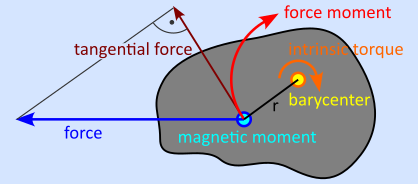
Sketch of force and torques acting on magnetic moment. — Sketch of force and torque acting on a magnetic moment that is part of a large mass system.#

Freely floating magnets: The pivot is the center of mass (barycenter). If the magnet has homogeneous mass density the barycenter coincides with the centroid (geometric center).
Mounted magnets: The pivot is given by the barycenter of the larger mass system on which the magnet is mounted, or simply by a mechanical attachment point like an axle, bearing, or hinge.

Input for pivot:

pivot='centroid': this is the default value and selects the geometric center of the target as pivot.
pivot=(x, y, z): any position can be specified as pivot point.
pivot=None: only the intrinsic magnetic torque contribution is computed.

Example: electric motor

The following example demonstrates how pivot point selection affects torque calculations in an electric motor configuration, where a permanent magnet mounted on a rotor interacts with current-carrying stator coils:

import numpy as np
import magpylib as magpy

# Set numpy print format
np.set_printoptions(formatter={"float": "{:.2e}".format})

# Rotor magnet
cube = magpy.magnet.Cuboid(
    dimension=(0.2, 0.2, 0.2), polarization=(0, 0, 1), meshing=1000
)

# Stator coils
loop1 = magpy.current.Circle(diameter=0.2, current=1e3, position=(0.1, 0, 0.15))
loop2 = magpy.current.Circle(diameter=0.2, current=-1e3, position=(-0.1, 0, 0.15))
stator = loop1 + loop2  # Collection of currents

# Compare torques for different pivot points
pivot_points = [None, "centroid", (0, 0, -0.5), (0, 0, -1)]
pivot_labels = ["Intrinsic only", "Centroid", "Axle at z=-0.5", "Axle at z=-1.0"]

for pivot, label in zip(pivot_points, pivot_labels):
    F, T = magpy.getFT(stator, cube, pivot=pivot)

    print(f"{label}:" f"  Force:  {np.round(F, 1)} N" f"  Torque: {np.round(T, 1)} N*m")

# Intrinsic only:
#   Force:  [80.6 -0.   0. ] N
#   Torque: [0.  5.7 0. ] N*m
#
# Centroid:
#   Force:  [80.6 -0.   0. ] N
#   Torque: [ 0.   3.4 -0. ] N*m
#
# Axle at z=-0.5:
#   Force:  [80.6 -0.   0. ] N
#   Torque: [ 0.  43.7 -0. ] N*m
#
# Axle at z=-1.0:
#   Force:  [80.6 -0.   0. ] N
#   Torque: [ 0. 84. -0.] N*m

Key observations:

The magnetic force is independent of the pivot point selection. It depends only on the relative position and orientation between source and target.
Lever arm effect: Moving the pivot further away from the force application points (each cell center) increases the force moment proportionally (\(T = r \times F\)).
With pivot=None we can compute the intrinsic torque excluding the force moment. This result is unphysical, but useful for comparison with other software.

Meshing#

Force and torque computation is based on numerical discretization of target objects. The meshing parameter controls this discretization by specifying the target number of mesh cells, directly affecting both computational accuracy and performance. Higher meshing values mean more cells, better accuracy, but longer computation time.

Hint

Set meshing to an integer representing the target number of mesh cells. The algorithms will select optimal cell distributions (homogeneous cells with aspect ratio close to 1) close to (but often not exactly) your target meshing value.

Class-specific meshing rules

Sphere and Dipole: no meshing required (automatically uses 1 point at center for exact results)
Cuboid: accepts also tuple meshing=(n1, n2, n3) for explicit subdivision
Circle: minimum meshing=4 (requires at least 4 points around circumference)
Polyline: minimum meshing must equal or exceed the number of line segments

Mesh analysis with meshreport

Meshing finesse is critical for estimating computation effort and expected precision. By calling F,T = getFT(..., meshreport=True) you can print the number of mesh cells of each target.

import magpylib as magpy

# Source
dipole = magpy.misc.Dipole(moment=(0, 0, 1e6))

# Targets
c1 = magpy.magnet.Cylinder(dimension=(2, 1), polarization=(0, 0, 1), meshing=1)
c2 = magpy.magnet.Cylinder(dimension=(2, 1), polarization=(0, 0, 1), meshing=10)
c3 = magpy.magnet.Cylinder(dimension=(2, 1), polarization=(0, 0, 1), meshing=100)

# Compute (F,T) AND generate mesh report
F, T = magpy.getFT(dipole, [c1, c2, c3], meshreport=True)

# Mesh report:
#   Target Cylinder(id=2589596340240): 2 points
#   Target Cylinder(id=2589596291216): 20 points
#   Target Cylinder(id=2589596292176): 124 points

Key insight: The algorithm selects optimal cell distributions close to (but not exactly) your target meshing value.

Mesh analysis with return_mesh

Use meshes = getFT(..., return_mesh=True) to inspect the generated meshes and verify proper discretization. In this case getFT() will return a list of dictionaries with keys 'pts', 'moments' and 'cvecs' containing the meshes of each target instead of (F, T).

import numpy as np
import magpylib as magpy
import matplotlib.pyplot as plt

# Source
dipole = magpy.misc.Dipole(moment=(0, 0, 1e6))

# Targets with increasing mesh density
i0 = 1
t1 = magpy.current.Circle(diameter=1, current=i0, meshing=8)
t2 = magpy.current.Circle(diameter=2, current=i0, meshing=24)
t3 = magpy.current.Circle(diameter=3, current=i0, meshing=64)

# Return mesh data instead of forces
meshes = magpy.getFT(dipole, [t1, t2, t3], return_mesh=True)

# Visualize mesh
fig, ax = plt.subplots(subplot_kw={'projection': '3d'}, dpi=130)
ax.view_init(elev=90, azim=0)  # Top-down view

colors = ['red', 'blue', 'forestgreen']
for mesh, color in zip(meshes, colors):
    # Load mesh
    points = mesh["pts"]         # mesh points
    cvecs = mesh["cvecs"] / i0   # current path tangent vectors

    # Draw current segments
    start = points - cvecs / 2  # starting point of current path
    ax.quiver(
        start[:, 0], start[:, 1], start[:, 2],
        cvecs[:, 0], cvecs[:, 1], cvecs[:, 2],
        colors=np.random.rand(len(cvecs),3)*.7, # Random dark color for each segment
        arrow_length_ratio=0 # No arrow head
    )

    # Draw mesh points
    ax.scatter(*points.T, s=8, c=color)

ax.set_title('Mesh Visualization')
plt.tight_layout()
plt.show()

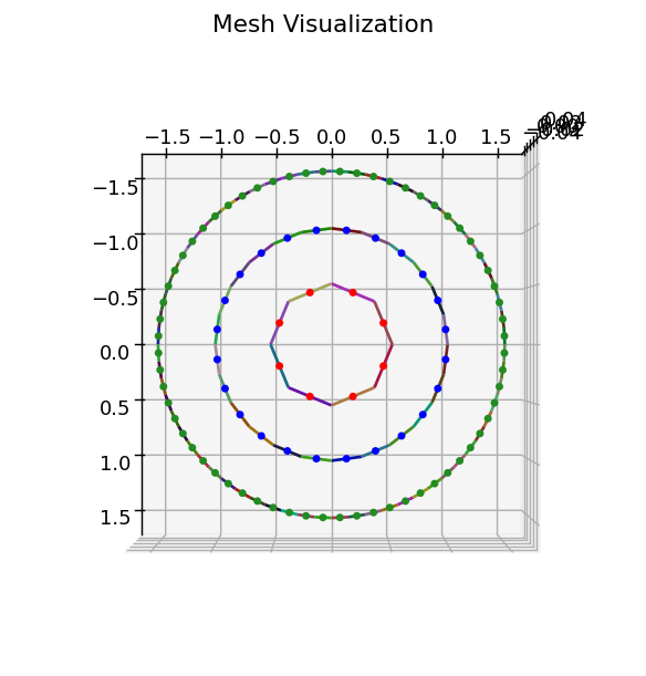
../../../_images/d2649660eb85dc1322195f46c1a5e3c5c2c02718518020ea4558a828a647f6cd.png

Key insights: return_mesh=True enables you to check the meshes in detail. Notice the uniform mesh point distribution and the finer finesse with increasing meshing parameter.

Finite Difference Gradient#

Magnet force computation requires the magnetic field gradient \(\nabla\vec{B}\), which Magpylib calculates using a finite difference scheme. The finite difference step size (absolute value in units (m)) is controlled by the eps parameter in getFT(). It is eps=1e-5 by default.

Good value for eps

as large as possible to avoid numerical cancellation
as small as possible for good gradient approximation

A good value can be 0.1 % of the smallest length in your system, but it’s best to simply try it out:

import numpy as np
import magpylib as magpy

# Set numpy print format
np.set_printoptions(formatter={"float": "{:.5e}".format})

# Example: magnet force computation with different eps values
cube1 = magpy.magnet.Cuboid(dimension=(1, 1, 1), polarization=(1, 0, 0))
cube2 = cube1.copy(position=(0.6, 0.7, 0.6), meshing=(4, 4, 4))

# Test different eps values
eps_values = [1e-2, 1e-3, 1e-4, 1e-5, 1e-20]

for eps in eps_values:
    F, T = magpy.getFT(cube1, cube2, eps=eps)
    print(F)

# [-1.32116e+04 1.96446e+04 4.72297e+04] - 1 correct digit
# [-1.21114e+04 1.94403e+04 4.62385e+04] - 2 correct digits
# [-1.20999e+04 1.94382e+04 4.62280e+04] - 4 correct digits
# [-1.20998e+04 1.94382e+04 4.62279e+04] - 6 correct digits
# [ 0.00000e+00 0.00000e+00 0.00000e+00] - no correct digits

Key observations: A good choice of eps balances good gradient approximation with low numerical noise.

Note

Current objects are not affected by the eps parameter as no gradient field is required for their force computation.

Convergence#

In general, the accuracy of the force computation improves with higher meshing values. Excluded from this rule are only Dipole and Sphere objects which give exact results without meshing.

The following example shows a computation that converges quickly with increasing mesh finesse. We employ reciprocity to compare to the exact solution.

import numpy as np
import magpylib as magpy

dipole = magpy.misc.Dipole(moment=(0, 0, 1e6), position=(1, 1, 1))
loop = magpy.current.Circle(diameter=1, current=1)

# Forward (exact)
F0, T0 = magpy.getFT(loop, dipole, pivot=(0, 0, 0))

# Backward (numerical), has opposite sign
for meshing in [8, 40, 200, 1000]:

    # Set meshing parameter
    loop.meshing = meshing

    # Compute backward force and torque
    F1, T1 = magpy.getFT(dipole, loop, pivot=(0, 0, 0))

    # Compute vectorwise relative error
    errF = np.linalg.norm(F1 + F0) / np.linalg.norm(F0)
    errT = np.linalg.norm(T1 + T0) / np.linalg.norm(T0)

    print(f"Meshing: {meshing:>4}, Force Error: {errF:.2e}, Torque Error: {errT:.2e}")

# Meshing:    8, Force Error: 1.02e-02, Torque Error: 3.93e-03
# Meshing:   40, Force Error: 3.82e-04, Torque Error: 8.30e-05
# Meshing:  200, Force Error: 1.53e-05, Torque Error: 3.31e-06
# Meshing: 1000, Force Error: 6.12e-07, Torque Error: 1.33e-07

Warning

Convergence behavior: Accuracy improvement is not always monotonic with mesh refinement. Some intermediate meshing values may temporarily show worse results before eventually converging to the correct solution.

Numerical sensitivity: Specific combinations of meshing and eps parameters can occasionally produce unreliable results due to numerical issues. Always test multiple parameter combinations to verify stability.

Summary - Best Practices#

A general ruleset for working properly with getFT() avoiding common pitfalls:

Single call of getFT()

# Good: Single vectorized call
F, T = magpy.getFT(sources, targets)  # Computes all forces at once

# Avoid: Multiple separate calls
for target in targets:
    F, T = magpy.getFT(sources, target)  # Inefficient!

Unless memory considerations: Memory usage scales with the total number of mesh points. The bottleneck is creating a large observer array (all mesh points + 6 finite difference points per magnet mesh point), and the subsequent call of getB(). For large systems, consider breaking into smaller batches.

Exploit reciprocity:

# Efficient: Use Dipole as target (1 mesh point)
F, T = magpy.getFT(cube, dipole)

# Less efficient: Use complex object as target (many mesh points)
F, T = magpy.getFT(dipole, cube)  # Requires meshing the cube

Verify convergence: Ideally, vary both meshing and eps parameters for testing convergence.

# Test multiple mesh densities
meshings = [50, 100, 200]
for m in meshings:
    target.meshing = m
    F, T = magpy.getFT(source, target)
    # Compare results...