Method of Images#
The method of images is a classical technique from electrostatics that can also be used in magnetostatics to obtain analytical solutions in the presence of highly permeable materials. In this example we show how it can be applied with Magpylib.
Textbook Fundamentals#
For the correct application of the method of images several requirements must be satisfied:
Linearity of the Governing Equation: The scalar potential \( \phi \) must satisfy a linear partial differential equation such as the Poisson equation:
\[\Delta \phi(\vec{r}) = -\frac{\rho(\vec{r})}{\varepsilon}\]where \( \Delta = \nabla \cdot \nabla \) is the Laplace operator, \( \varepsilon \) is a constant permittivity, and \( \rho(\vec{r}) \) is the source distribution (=charges) that generates the field.
Homogeneity in the Region of Interest: The method of images is only applicable in charge-free regions, where the governing equation reduces to Laplace’s equation:
\[\Delta \phi(\vec{r}) = 0\]Simple Geometry and Boundary Conditions: The boundary must be geometrically simple – typically a plane, sphere, or infinite cylinder. On the surface a simple boundary condition, like constant potential, must hold, and natural boundaries must be satisfied at infinity. This implies that the resulting gradient field \( \vec{F} = -\nabla \phi \) is normal to the boundary surface, and decays at infinity.
Applicability of the Uniqueness Theorem: The method relies on the uniqueness theorem: if a solution satisfies both the differential equation and the boundary conditions, it is the only physically valid solution in that region.
When all of these criteria are satisfied, the potential field in the region of interest can be constructed as the superposition of the original source distribution \( \rho(\vec{r}) \) and an image source \( \rho^*(\vec{r}) \), which is a mirror reflection of the original source across the boundary.
Method of Images in Magnetostatics#
In magnetostatics, the method of images can be applied in the presence of highly permeable (\(\mu_r \gg 1\)) soft magnetic materials. In such materials, the magnetic moments can rotate freely and align in a way that completely suppresses the \( \vec{H} \)-field inside the body. As a result, the field is forced to be normal to the material’s surface, making simple planar boundaries ideal for image constructions and satisfying condition (3).
Furthermore:
In magnetostatics, the magnetic field \( \vec{H} \) can be expressed as the gradient of a magnetic scalar potential: \(\vec{H} = -\nabla \phi_m \) satisfying condition (1), provided we are in regions without free currents.
Uniformly magnetized bodies, like the permanent magnets implemented in Magpylib, can be modeled using magnetic surface charges. This means that condition (2) is fulfilled everywhere except on these surfaces.
The uniqueness theorem applies to all well-posed magnetostatic problems, satisfying condition (4).
This means that magnets and currents can be mirrored across a highly permeable surface to compute the magnetic field outside the material. For magnetization, the normal component is preserved and the tangential components are inverted. For currents, the tangential component is preserved, while the normal component is inverted, as illustrated in the image below.

Sketch of how the image method works in magnetostatics#
Note: Do not confuse this with the case of superconductors, where the method of images is also applicable — but for entirely different physical reasons (perfect diamagnetism rather than high permeability).
Example Applications#
The method of images does not require an idealized, infinitely permeable half-space. In practice, even thin (not too thin though), finite soft-magnetic layers—such as the soft-magnetic backs of inductors or magnetic shielding plates—can provide sufficient contrast for the image method. In addition, even relatively low permeabilities \(\mu_r> 10\) or \(\mu_r>100\) result in good agreement between experiment and theory.
One practical use case is shown in the example on magnetic scale structures, such as pole wheels, where a soft-magnetic backing enhances the field of out-of-plane magnetized patterns.
Another application is the computation of holding forces between permanent magnets and soft magnetic surfaces.
Example of the Magnetic Image Method#
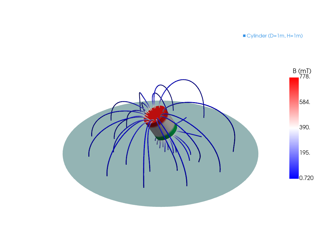
In the following example, a permanent magnet is placed above a planar magnetic shield located in the xy-plane. The mirror image is modeled as a second magnet, placed below the plane according to the method of images. We then compute the magnetic field in the upper half-space.
For field visualization, we use PyVista streamlines. Notice how the field lines are perpendicular to the mirror surface at the interface — consistent with the boundary conditions imposed by a highly permeable material.
2026-05-16 11:50:50.911 ( 1.377s) [ 7F09196FCB80]vtkXOpenGLRenderWindow.:1460 WARN| bad X server connection. DISPLAY=
/tmp/ipykernel_1810/2549158571.py:71: UserWarning: Using static image for notebook display.
Install trame for interactive backends: pip install "pyvista[jupyter]"
  pl.show()