Current Sheets

A current sheet is an idealized surface over which an electric current flows continuously. Instead of current being distributed throughout a volume, it is concentrated in an infinitesimally thin layer, described by a surface current density \(\vec{j}\) with units of A/m.

Magpylib provides an implementation for computing the magnetic field generated by an arbitrary current flowing along a triangular surface. This feature allows the construction of complex surface current distributions through superposition of multiple triangular elements.

The object-oriented interface offers two dedicated classes for this purpose:

---

Triangle Strip

The TriangleStrip class provides a convenient way to construct a current-carrying strip, band, or ribbon by simply supplying a sequence of vertices. These vertices should follow the alternating top-and-bottom pattern described in the class documentation.

Show code cell source

Hide code cell source

import numpy as np
import magpylib as magpy

def mobis_strip_vertices(w):
    """Generate vertices for a Möbius strip at a given width w."""
    U = np.linspace(0, 4 * np.pi, 100)
    X = (1 + w * np.cos(U / 2)) * np.cos(U)
    Y = (1 + w * np.cos(U / 2)) * np.sin(U)
    Z = w * np.sin(U / 2)
    return np.array([X, Y, Z]).T

# Create a mobius current strip
verts = np.zeros((200, 3))
verts[::2] = mobis_strip_vertices(0)
verts[1::2] = mobis_strip_vertices(0.4)

strip = magpy.current.TriangleStrip(
    vertices=verts,
    current=1,
    style_label="Mobius Current Sheet",
)

strip.show(backend="plotly")

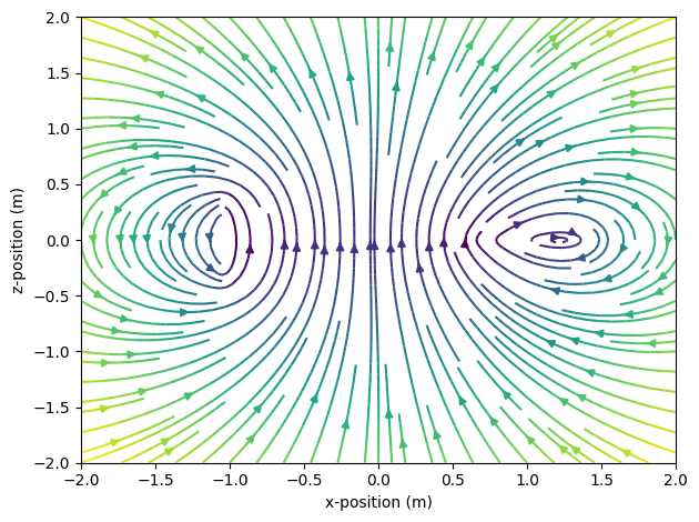
We visualize the magnetic field of this current strip in the x–z plane, following the Matplotlib streamplot example. Notice how the streamlines differ: on the left side, where the strip is oriented upright, the field appears distinctly different from the right side, where the strip lies in-plane.

Show code cell source

Hide code cell source

# ... continuation from above

import matplotlib.pyplot as plt

# Create a Matplotlib figure
fig, ax = plt.subplots()

# Create an observer grid in the xz-symmetry plane
ts = np.linspace(-2, 2, 40)
grid = np.array([[(x, 0, z) for x in ts] for z in ts])
X, _, Z = np.moveaxis(grid, 2, 0)

# Compute the B-field of the mobius strip on the grid
B = strip.getB(grid)
Bx, _, Bz = np.moveaxis(B, 2, 0)

# Display the B-field with streamplot
splt = ax.streamplot(X, Z, Bx, Bz,
    density=1.5,
    color=np.log10(np.linalg.norm(B, axis=2)),
    cmap="viridis_r",
)

# Figure styling
ax.set(
    xlabel="x-position (m)",
    ylabel="z-position (m)",
)

plt.tight_layout()
plt.show()

Current strips can also be used to create complex magnet prisms using the Equivalent Current Method.

---

Triangle Sheet

The TriangleSheet class is used to construct arbitrary current sheets from a collection of individual triangle elements, each carrying its own specified surface current density. This enables detailed modeling of complex surface current distributions with good control over geometry and current flow.

If you already have a triangulated surface along with corresponding current density vectors—e.g., from a finite element simulation—this data can be directly passed to the TriangleSheet class.

In the following example, we generate a triangular mesh covering a square region and define a spatially varying current density using a custom function.

Show code cell source

Hide code cell source

import numpy as np
import magpylib as magpy

# Parameters
n = 11  # number of points per side (discretization)
ts = np.linspace(-1, 1, n)

# Generate grid of vertices in the x-y plane
vertices = np.array([(x, y, 0) for x in ts for y in ts])

# Generate triangle faces using row-major indexing
faces = []
for i in range(n - 1):
    for j in range(n - 1):
        idx = j + i * n
        faces.append((idx, idx + n, idx + n + 1))
        faces.append((idx, idx + n + 1, idx + 1))
faces = np.array(faces, dtype=int)

# Define a current density function
def current_density(positions):
    """Return current density vectors for given positions."""
    x, y, _ = positions.T
    return np.stack([y, -x, np.zeros_like(x)], axis=1)

# Compute current densities at triangle centers
face_centers = np.mean(vertices[faces], axis=1)
cds = current_density(face_centers)

# Create a TriangleSheet object
sheet = magpy.current.TriangleSheet(
    current_densities=cds,
    vertices=vertices,
    faces=faces,
    style_mesh_grid_show=True,
    style_mesh_grid_line_width=0.5,
    style_direction_color='b',
    style_direction_symbol='cone',
)

# Visualize in Plotly
sheet.show(backend="plotly")

This setup corresponds to a circular surface current with increasing amplitude towards the edges of a rectangular sheet. Notice that we can tune the mesh styling.

Now we use a pixel field quiver plot to visualize the resulting magnetic field with minimal effort:

Show code cell source

Hide code cell source

# ... continuation from above

# Create an observer grid in the xz-symmetry plane
xs = np.linspace(-1.5, 1.5, 30)
ys = np.linspace(-1, 1, 20)
grid = np.array([[(x, 0, z) for x in xs] for z in ys])

# Create a sensor with pixel array and pixel field style
sens = magpy.Sensor(
    pixel=grid,
    style_pixel_field_source='B',
    style_pixel_field_symbol='arrow3d',
    style_pixel_field_sizescaling='uniform',
    style_pixel_field_colormap='Plasma',
)

# Display the sensor and magnet using the Plotly backend
magpy.show([sheet, sens], backend="plotly", style_legend_show=False)

We observe that the B-field closely resembles the field of a classical current loop. Possibly this is the result of the current’s increase in amplitude with distance from the center of the sheet.