Floating Magnets#
The examples here require installaion of the magpylib-force package. See also the magpylib-force documentation.
Formalism#
With force and torque we can compute how a magnet moves in a magnetic field by solving the equations of motion,
with force \(\vec{F}\), momentum \(\vec{p}\), torque \(\vec{T}\) and angular momentum \(\vec{L}\).
We implement a first order semi-implicit Euler method that is used to compute planetary motion. The algorithm splits the computation into small subsequent time-steps \(\Delta t\), resulting in the following equations for the position \(\vec{s}\), the velocity \(\vec{v} = \dot{\vec{s}}\), the rotation angle \(\vec{\varphi}\) and the angular velocity \(\vec{\omega}\),
Magnet and Coil#
In the following example we show an implementation of the proposed Euler scheme. A cubical magnet is accelerated by a current loop along the z-axis as show in the following sketch:
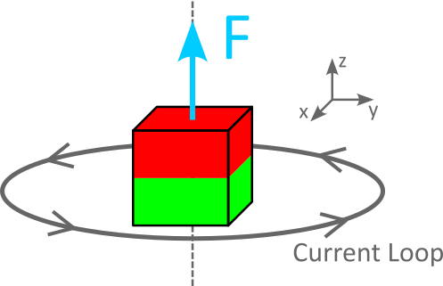
A cubical magnet is accelerated by a current loop.#
Due to the symmetry of the problem there is no torque so we solve only the translation part of the equations of motion.
In the beginning, the magnet is at rest and slightly displaced in z-direction from the center of the current loop. With time the magnet is accelerated and it’s z-position is displayed in the figure below.
import numpy as np
import matplotlib.pyplot as plt
import magpylib as magpy
from magpylib_force import getFT
from scipy.spatial.transform import Rotation as R

def timestep(source, target, dt):
    """
    Apply translation-only Euler-sceme timestep to target.

    Parameters:
    -----------
    source: Magpylib source object that generates the magnetic field

    target: Magpylib target object viable for force computation. In addition,
        the target object must have the following parameters describing
        the motion state: v (velocity), m (mass)

    dt: Euler scheme length of timestep
    """

    # compute force
    F, _ = getFT(source, target)

    # compute/set new velocity and position
    target.v = target.v + dt/target.m * F
    target.position = target.position + dt * target.v

# Current loop that generates the field
loop = magpy.current.Circle(diameter=10e-3, current=10)

# Magnets which are accelerated in the loop-field
cube1 = magpy.magnet.Cuboid(dimension=(5e-3,5e-3,5e-3), polarization=(0,0,1))
cube1.meshing=(3,3,3)
cube2 = cube1.copy(polarization=(0,0,-1))

# Compute motion
for cube, lab in zip([cube1, cube2], ["attractive", "repulsive"]):

    # Set initial conditions
    cube.m = 1e-3
    cube.position=(0,0,3e-3)
    cube.v = np.array([0,0,0])

    # Compute timesteps
    z = []
    for _ in range(100):
        z.append(cube.position[2]*1000)
        timestep(loop, cube, dt=1e-3)

    plt.plot(z, marker='.', label=lab)

# Graphic styling
plt.gca().legend()
plt.gca().grid()
plt.gca().set(
    title="Magnet motion",
    xlabel="timestep ()",
    ylabel="z-Position (mm)",
)
plt.show()
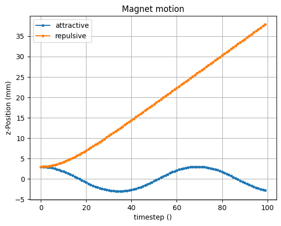
The simulation is made with two magnets with opposing polarizations. In the “repulsive” case (orange) the magnetic moment of magnet and coil are anti-parallel and the magnet is simply pushed away from the coil in positive z-direction. In the “attractive” case (blue) the moments are parallel to each other, and the magnet is accelerated towards the coil center. Due to inertia it then comes out on the other side, and is again attracted towards the center resulting in an oscillation.
Warning
This algorithm accumulates its error over time, which can be avoided by choosing smaller timesteps.
Two-body problem#
In the following example we demonstrate a fully dynamic simulation with two magnetic bodies that rotate around each other, attracted towards each other by the magnetic force, and repelled by the centrifugal force.
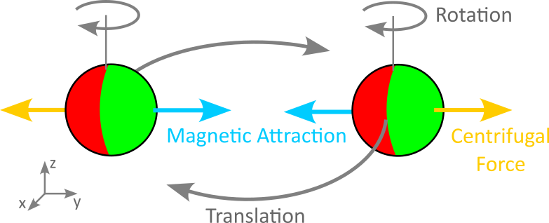
Two freely moving magnets rotate around each other.#
Contrary to the simple case above, we apply the Euler scheme also to the rotation degrees of freedom, as the magnets will change their orientation while they circle around each other.
import numpy as np
import matplotlib.pyplot as plt
import magpylib as magpy
from magpylib_force import getFT
from scipy.spatial.transform import Rotation as R

def timestep(source, target, dt):
    """
    Apply full Euler-sceme timestep to target.

    Parameters:
    -----------
    source: Magpylib source object that generates the magnetic field

    target: Magpylib target object viable for force computation. In addition,
        the target object must have the following parameters describing
        the motion state: v (velocity), m (mass), w (angular velocity),
        I_inv (inverse inertial tensor)

    dt: Euler scheme length of timestep
    """
    # compute force
    F, T = getFT(source, target)

    # compute/set new velocity and position
    target.v = target.v + dt/target.m * F
    target.position = target.position + dt * target.v

    # compute/set new angular velocity and rotation angle
    target.w = target.w + dt*target.orientation.apply(np.dot(target.I_inv, target.orientation.inv().apply(T)))
    target.orientation = R.from_rotvec(dt*target.w)*target.orientation


v0 = 5.18   # init velocity
steps=505   # number of timesteps
dt = 1e-2   # timstep size

# Create the two magnets and set initial conditions
sphere1 = magpy.magnet.Sphere(position=(5,0,0), diameter=1, polarization=(1,0,0))
sphere1.meshing = 5
sphere1.m = 2
sphere1.v = np.array([0, v0, 0])
sphere1.w = np.array([0, 0, 0])
sphere1.I_inv = 1 * np.eye(3)

sphere2 = sphere1.copy(position=(-5,0,0))
sphere2.v = np.array([0,-v0, 0])

# Solve equations of motion
data = np.zeros((4,steps,3))
for i in range(steps):
    timestep(sphere1, sphere2, dt)
    timestep(sphere2, sphere1, dt)

    # Store results of each timestep
    data[0,i] = sphere1.position
    data[1,i] = sphere2.position
    data[2,i] = sphere1.orientation.as_euler('xyz')
    data[3,i] = sphere2.orientation.as_euler('xyz')

# Plot results
fig, (ax1,ax2) = plt.subplots(2,1,figsize=(10,5))

for j,ls in enumerate(["-", "--"]):

    # Plot positions
    for i,a in enumerate("xyz"):
        ax1.plot(data[j,:,i], label= a + str(j+1), ls=ls)

    # Plot orientations
    for i,a in enumerate(["phi", "psi", "theta"]):
        ax2.plot(data[j+2,:,i], label= a + str(j+1), ls=ls)

# Figure styling
for ax in fig.axes:
    ax.legend(fontsize=9, loc=6, facecolor='.8')
    ax.grid()
ax1.set(
    title="Floating Magnet Ringdown",
    ylabel="Positions (m)",
)
ax2.set(
    ylabel="Orientations (rad)",
    xlabel="timestep ()",
)
plt.tight_layout()
plt.show()
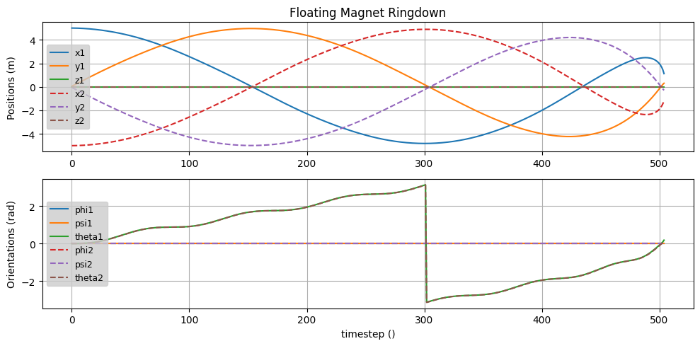
In the figure one can see, that the initial velocity is chosen so that the magnets approach each other in a ringdown-like behavior. The magnets are magnetically locked towards each other - both always show the same orientation. However, given no initial angular velocity, the rotation angle is oscillating several times while circling once.
A video is helpful in this case to understand what is going on. From the computation above, we build the following gif making use of this export-animation tutorial.
Animation of above simulated magnet ringdown.#