Field Computation#
The following is a detailed technical documentation of Magpylib field computation. The tutorial Computing the Field shows good practices and illustrative examples.
Object-oriented interface#
The object-oriented interface relies on the idea that sources of the magnetic field and observers thereof are created as Python objects which can be manipulated at will, and called for field computation. This is done via four top-level functions getB, getH, getJ and, getM,
magpylib.getB(sources, observers, squeeze=True, pixel_agg=None, output="ndarray")
magpylib.getH(sources, observers, squeeze=True, pixel_agg=None, output="ndarray")
magpylib.getJ(sources, observers, squeeze=True, pixel_agg=None, output="ndarray")
magpylib.getM(sources, observers, squeeze=True, pixel_agg=None, output="ndarray")
that compute the respective fields B (B-field), H (H-field), J (polarization) or M (magnetization) generated by sources as seen by the observers in their local coordinates. sources can be any Magpylib source object (e.g. magnets) or a flat list thereof. observers can be an array of position vectors with shape (n1,n2,n3,...,3), any Magpylib observer object (e.g. sensors), or a flat list thereof. The following code shows a minimal example for Magpylib field computation.
import magpylib as magpy

# Define source and observer objects
loop = magpy.current.Circle(current=1, diameter=.001)
sens = magpy.Sensor()

# Compute field
B = magpy.getB(loop, sens)

print(B)
#  --> [0.         0.         0.00125664]
For quick access, the functions getBHJM are also methods of all Magpylib objects, such that the sources or observers input is the object itself. The above example can be continued as
# Call getB as method of loop
B = loop.getB(sens)

# Call getB as method of loop
B = sens.getB(loop)
with the same result for B.
By default, getB returns the B-field in units of T, getH the H-field in units of A/m, getJ the magnetic polarization in T and, getM the magnetization in A/m, assuming that all inputs are given in SI units as described in the docstrings.
Hint
In reality, getB is proportional to the polarization input and therefore returns the same unit. For example, with polarization input in mT, getB will return mT as well. At the same time when the magnetization input is kA/m, then getH returns kA/m as well. The B/H-field outputs are related to a M/J-inputs via a factor of \(µ_0\).
The output of a field computation magpy.getB(sources, observers) is by default a NumPy array of shape (l, m, k, n1, n2, n3, ..., 3) where l is the number of input sources, m the (maximal) object path length, k the number of observers, n1,n2,n3,... the sensor pixel shape or the shape of the observer position array input and 3 the three magnetic field components \((B_x, B_y, B_z)\).
squeeze: If True (default) all axes of length 1 in the output (e.g. only a single source) are squeezed.pixel_agg: Select a compatible NumPy aggregator function (e.g."min","mean") that is applied to the output. For example, withpixel_agg="mean"the mean field of all observer points is returned. With this option it is possible to supplygetBHJMwith multiple observers that have different pixel shapes.output: Change the output format. Options are"ndarray"(default, returns a NumPy ndarray) and"dataframe"(returns a 2D-table Pandas DataFrame).
Note
Magpylib collects all inputs (object parameters), and vectorizes them for the computation which reduces the computation time dramatically for large inputs.
Try to make all field computations with as few calls to getBHJM as possible. Avoid Python loops at all costs!
Functional interface#
Users can bypass the object oriented functionality of Magpylib and instead compute the field for n given parameter sets. This is done by providing the following inputs to the top level functions getB, getH, getJ and, getM.
sources: a string denoting the source type. Allowed values are the Magpylib source class names, see The Magpylib Classes.observers: array-like of shape (3,) or (n,3) giving the observer positions.kwargs: a dictionary with inputs of shape (x,) or (n,x). Must include all mandatory class-specific inputs. By default,position=(0,0,0)andorientation=None(=unit rotation).
All “scalar” inputs of shape (x,) are automatically tiled up to shape (n,x) to create a set of n computation instances. The field is returned in the shape (n,3). The following code demonstrates the functional interface.
import numpy as np
import magpylib as magpy
# All inputs and outputs in SI units

# Compute the cuboid field for 3 input instances
N = 3 # number of instances
B = magpy.getB(
    sources='Cuboid',
    observers=np.linspace((0,0,1), (0,0,3), N),
    dimension=np.linspace((1,1,1), (3,3,3),3, N),
    polarization=(0,0,1),
)

# This example demonstrates the scale invariance
print(B)
#  --> [[0.         0.         0.13478239]
#       [0.         0.         0.13478239]
#       [0.         0.         0.13478239]]
Note
The functional interface is potentially faster than the object oriented one if users know how to generate the input arrays efficiently with numpy (e.g. np.arange, np.linspace, np.tile, np.repeat, …).
Core interface#
At the heart of Magpylib lies a set of core functions that are our implementations of analytical field expressions found in the literature, see Physics and Computation. Direct access to these functions is given through the magpylib.core subpackage which includes,
magnet_cuboid_Bfield( observers, dimensions, polarizations)
magnet_cylinder_axial_Bfield( z0, r, z)
magnet_cylinder_diametral_Hfield( z0, r, z, phi)
magnet_cylinder_segment_Hfield( observers, dimensions, magnetizations)
magnet_sphere_Bfield(observers, diameters, polarizations)
current_circle_Hfield(r0, r, z, i0)
current_polyline_Hfield(observers, segments_start, segments_end, currents)
dipole_Hfield(observers, moments)
triangle_Bfield(observers, vertices, polarizations)
All inputs must be NumPy ndarrays of shape (n,x). Details can be found in the respective function docstrings. The following example demonstrates the core interface.
import numpy as np
import magpylib as magpy
# All inputs and outputs in SI units

# Prepare input
z0 = np.array([1,1])
r  = np.array([1,1])
z  = np.array([2,2])

# Compute field with core functions
B = magpy.core.magnet_cylinder_axial_Bfield(z0=z0, r=r, z=z).T

print(B)
#  --> [[0.05561469 0.         0.06690167]
#       [0.05561469 0.         0.06690167]]
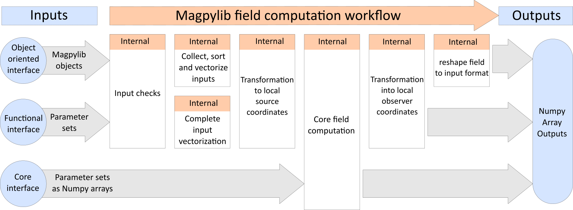
Field computation workflow#
The Magpylib field computation internal workflow and different approaches of the three interfaces is outlined in the following sketch.