Magnetic Scales

The following examples we demonstrate how analytical models can be used to simulate magnetic scales. Some measurements and simulations are taken from the publication [P2-OSM+25], which provides a more in-depth discussion for those interested in the underlying theory and experimental validation.

---

Background

Magnetic scales are patterned arrays of permanent magnets—typically with alternating magnetization directions—engineered to produce predictable magnetic fields along a line or surface. They are commonly implemented as pole wheels, magnetic strips, or tracks, and are used in combination with field sensors such as Hall-effect or magnetoresistive sensors for precise position and motion detection.

Typical applications include rotary and linear encoders in robotics and automation, as well as speed and position sensing in industrial systems. Because the measurement is contactless and robust, magnetic scales are well suited for environments with dust, vibration, or temperature extremes where traditional sensing methods might fail. They are also widely used in the automotive industry—for example, in angle detection systems for steering or throttle control.

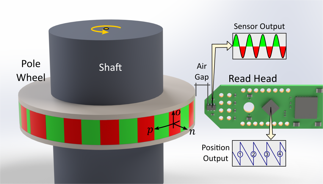
Sketch of a rotary encoder with pole wheel and magnetic sensor. The sensor detects an oscillating magnetic field, which is then transformed into a linear output by a microcontroller.

---

Encoder Terminology - INNOMAG Guideline

The INNOMAG e.V. Guideline is a revision of the DIN SPEC 91411[P2-DIN22], a norm for unifying magnetic encoder technical representation and nomenclature.

• The coordinates \(p\) (wheel rotation angle or associated arc length), \(o\) (axial length), and \(n\) (radial distance from wheel surface) are used for relative positioning to the pole wheel.

• The magnetic field profile \( B_\alpha(\vec{c}) \) refers to the \(\alpha\)-component of the \(\textit{B}\)-field, \( \alpha \in \{p, n, o\} \), along a path \(\vec{c}\). Along a track it is commonly denoted by \( B_\alpha(p) \).

• Magnetic poles are regions above the wheel surface, where a component of the magnetic field does not change its sign in \(p\) direction and does not undercut a threshold in \(o\) direction. This definition contrasts the classical physics usage, which vaguely refers to surface areas on a magnet. The pole length \(\ell_P\) denotes the distance between subsequent zero-crossings along \(p\) direction. Poles are typically characterized by single magnetic peaks corresponding to the \(i\)th minima and maxima of the field profile \(B_\alpha(p)\) with magnitudes \(B_{\alpha, A}^i\) and mean value \(\bar{B}_{\alpha, A}\).

• Magnetic zones are volumes of permanently magnetized material with comparable magnetic polarization density vectors that reflect the magnetization periodicity. Their characteristic dimensions are termed zone length \(\ell_Z\) in \(p\) direction, zone width \(w_Z\) in \(o\) direction, both defined on the zone surface, and zone depth \(d_Z\) in \(n\) direction.

The magnetic working distance \( n^{\text{mag}} \) is the distance between the surface of the magnetic zones and the sensor’s sensitive elements. It differs from the air gap \( n^{\text{mech}} \), defined as the distance between sensor housing and wheel surface.

The following figure provides a schematic overview of the terminology.

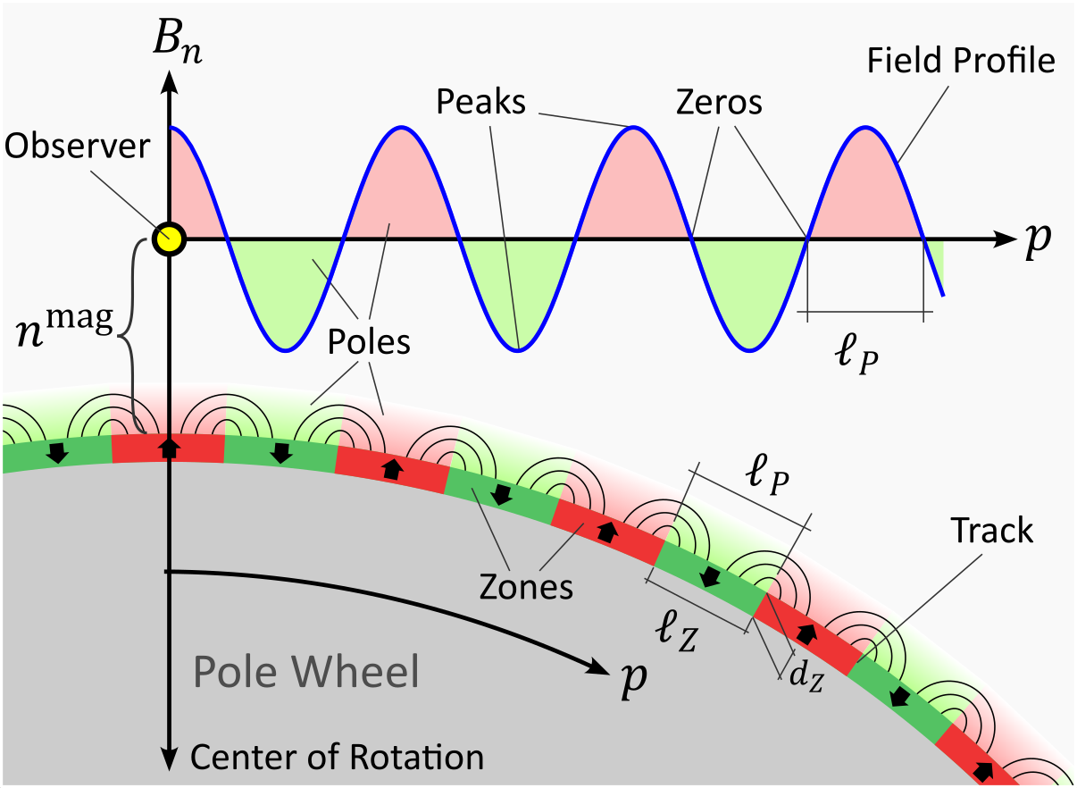
Visualization of encoder terminology.

---

Magnetic Scale Taxonomy

This taxonomy provides an overview of the various types of commonly used magnetic scales and classifies them according to their design and application. The diagram shown below is reproduced from the German standard DIN SPEC 91411[P2-DIN22], and a translated version is expected to be included in the upcoming INNOMAG Guidelines.

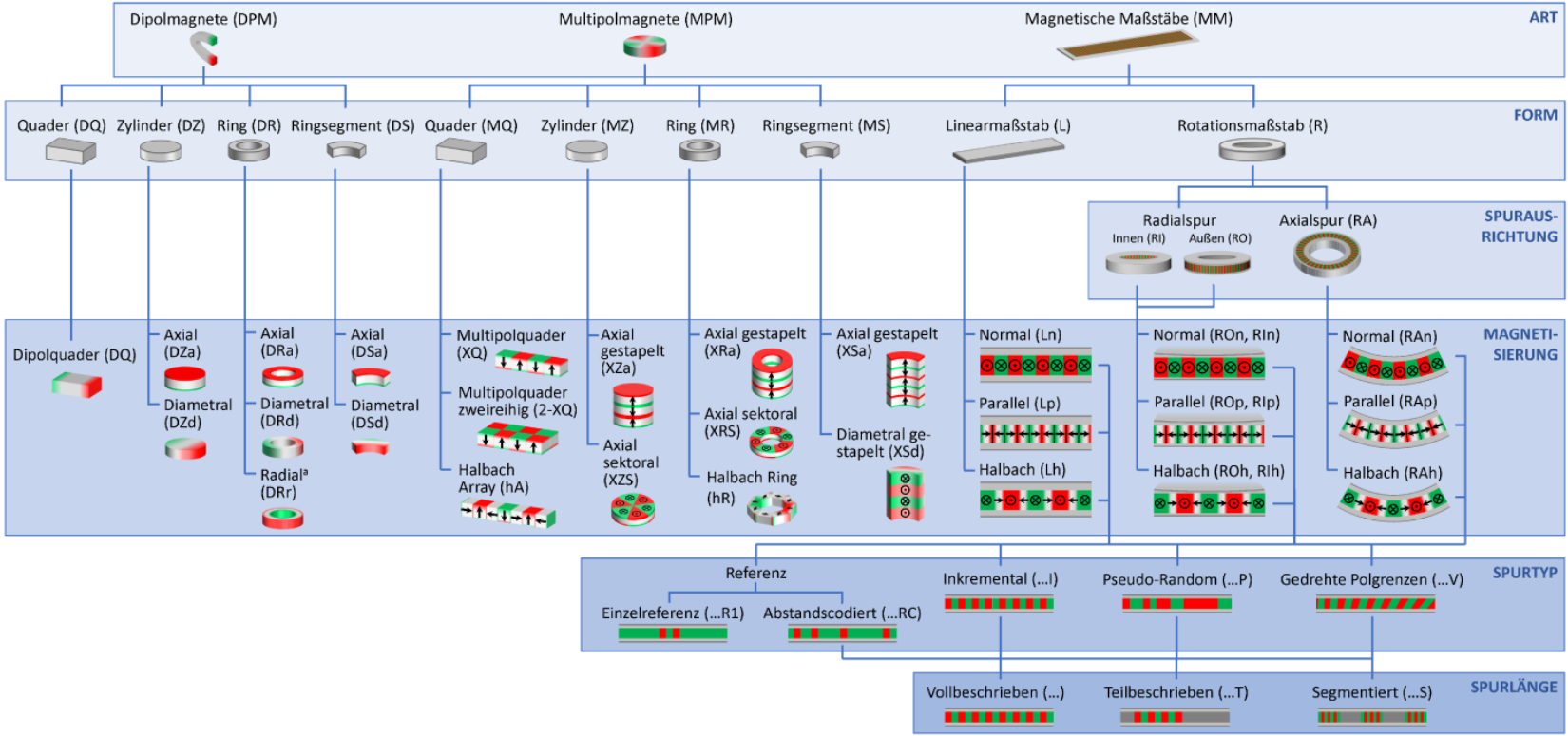
Taxonomy of magnetic scales as defined in DIN SPEC 91411.

---

Ideal-Typical Models

Ideal-typical models of magnetic scales refer to simplified magnetization patterns constructed from homogeneously magnetized geometric primitives. These models serve as idealized representations of real magnetic structures and can closely approximate the magnetic fields observed in practice. This is demonstrated in the figure below, which compares an experimental measurement of an incremental ROn scale with a simulation based on an ideal-typical model built using Magpylib.

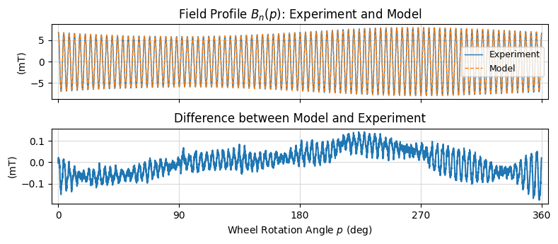
Comparison between experimental measurement and simulation based on an ideal-typical Magpylib model.

The mean deviation between simulation and experiment is below \( 0.7\% \bar{B}_A\), approaching demagnetization limits, and often surpassing experimental precision and magnet fabrication tolerances.

Despite their effectiveness for capturing key qualitative and quantitative effects in encoder systems, it is important to emphasize that ideal-typical models may not faithfully represent the true underlying polarization distribution.

---

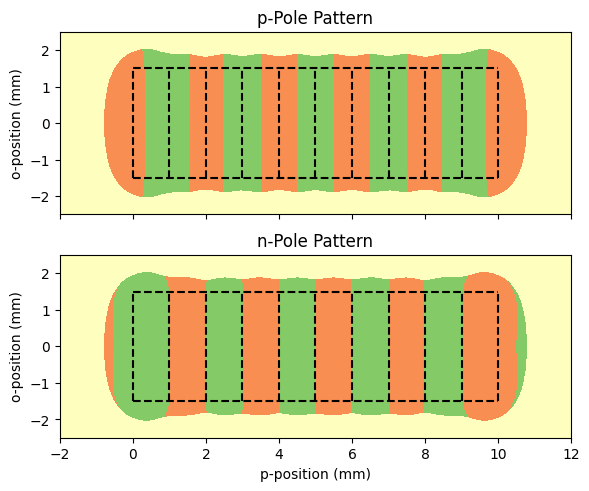
Linear Scale Model

In the following example, we construct a typical linear magnetic scale with 10 alternating zones, using ferrite material with a remanent flux density of approximately 0.3 T. See the magnet modeling tutorial for how remanence relates to the polarization input in Magpylib.

We choose an out-of-plane zone pattern with typical zone length 1 mm, zone width 3 mm and zone depth 0.3 mm. The following coordinate assignment convention between Magpylib and typical encoder notation is used: x ⇄ p (position along the scale), y ⇄ o (orthogonal in the scale plane), and z ⇄ n (normal to the scale surface).

Show code cell source

Hide code cell source

import numpy as np
import magpylib as magpy

# Parameters
zone_number = 10
zone_length = 1e-3
zone_width = 3e-3
zone_depth = 0.3e-3

# Create linear magnetic scale with alternating magnetization
scale = magpy.Collection(style_label='LnI-Scale')
for i in range(zone_number):
    scale.add(magpy.magnet.Cuboid(
        dimension=(zone_length, zone_width, zone_depth),
        polarization=(0, 0, 0.3 * (-1)**i),  # 0.3 T up/down
        position=((i + 0.5) * zone_length, 0, -zone_depth / 2),
    ))

# Visualize with Plotly backend
scale.show(backend='plotly')

The scale is constructed so that the beginning of the first magnetic zone lies at \( x = p = 0 \), and the top surface of the scale lies in the xy-plane.

Next, we compute and visualize the pole patterns of the \(n\)- and \(p\)-components of the magnetic field at a working distance of 0.5 mm, using contour plots.

To aid interpretation:

• A field amplitude threshold of 5 mT is applied: regions below this value are highlighted with a yellow contour.

• The underlying magnetization zone pattern is overlaid as dashed lines for reference.

Show code cell source

Hide code cell source

import matplotlib.pyplot as plt

# Parameters
Bthresh = 5  # mT threshold for pole detection
cmap = 'RdYlGn'

# Create grid for magnetic field calculation
ps = np.linspace(-2e-3, zone_number*zone_length + 2e-3, 100)
os = np.linspace(-zone_width/2-1e-3, zone_width/2+1e-3, 20)
grid = [[(p, o, 0.5e-3) for p in ps] for o in os]

# Compute magnetic field
B = scale.getB(grid) * 1000  # convert to mT
B_amp = np.linalg.norm(B, axis=-1)

# Plot setup
fig, (ax1, ax2) = plt.subplots(2, 1, figsize=(6, 5), sharex=True)
P, O = np.meshgrid(ps*1e3, os*1e3) # convert to mm

# Plot p-component (x) and threshold contours
ax1.contourf(P, O, B[..., 0], levels=1, cmap=cmap)
ax1.contourf(P, O, B_amp, levels=[-1e3, Bthresh], cmap=cmap)

# Plot n-component (z) and threshold contours
ax2.contourf(P, O, B[..., 2], levels=1, cmap=cmap)
ax2.contourf(P, O, B_amp, levels=[-1e3, Bthresh], cmap=cmap)

# Overlay zone outlines
zl = zone_length * 1e3  # convert to mm
zw = zone_width * 1e3  # convert to mm
for ax in fig.axes:
    for i in range(zone_number+1):
        ax.plot([i*zl]*2, [-zw/2, zw/2], 'k--')
    ax.plot([0, zone_number*zl], [-zw/2]*2, 'k--')
    ax.plot([0, zone_number*zl], [ zw/2]*2, 'k--')

# Labels and styling
ax1.set(title='p-Pole Pattern', ylabel='o-position (mm)', aspect='equal')
ax2.set(title='n-Pole Pattern', xlabel='p-position (mm)', ylabel='o-position (mm)', aspect='equal')

plt.tight_layout()
plt.show()

---

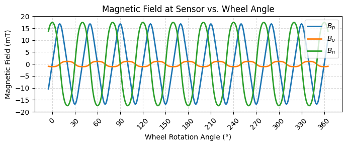
Polewheel Model

The following example demonstrates how to construct a RAn polewheel with an incremental track consisting of 18 magnetized zones. Each zone is modeled as a magnetized cylindrical segment with alternating out-of-plane polarization. Similar wheels are commonly used for rotary encoders.

Show code cell source

Hide code cell source

import numpy as np
import magpylib as magpy

# Parameters
zone_number = 18
track_radius = 5e-3   # Inner radius of track (m)
zone_width = 2e-3     # Radial width of each zone (m)
zone_depth = 0.3e-3   # Axial depth of each magnet (m)
J0 = 0.3              # Polarization magnitude (T)

# Create polewheel with alternating out-of-plane polarization
wheel = magpy.Collection(style_label='RAn-Wheel')
angle_per_zone = 360 / zone_number

for i in range(zone_number):
    start_angle = i * angle_per_zone
    end_angle = (i + 1) * angle_per_zone
    pol = (0, 0, J0 * (-1)**i)
    segment = magpy.magnet.CylinderSegment(
        dimension=(track_radius, track_radius + zone_width, zone_depth, start_angle, end_angle),
        polarization=pol,
    )
    wheel.add(segment)

# Visualize with Plotly
wheel.show(backend='plotly')

For this wheel, the zone length (measured at the center of the track) is approximately 2.1 mm. We compute and visualize the magnetic field components directly above the center of the track at a working distance of 1 mm (~1/2 zone length). The wheel is rotated from −5° to 365°, and the resulting field components at a fixed sensor location are shown as a function of the rotation angle.

Show code cell source

Hide code cell source

import matplotlib.pyplot as plt

# Define sensor directly above center of track at 1 mm distance
sensor = magpy.Sensor(position=(0, track_radius + zone_width/2, 1e-3))

# Define rotation of the wheel
angles = np.linspace(-5, 365, 371)  # in degrees
wheel.rotate_from_angax(angles, "z", start=0)

# Get magnetic field at the sensor (converted to mT)
Bp, Bo, Bn = wheel.getB(sensor).T * 1000

# Plot field components
fig, ax = plt.subplots(figsize=(7, 3))
ax.plot(angles, Bp, label=r'$B_p$', lw=2)
ax.plot(angles, Bo, label=r'$B_o$', lw=2)
ax.plot(angles, Bn, label=r'$B_n$', lw=2)

# Axis labels and styling
ax.set(
    title='Magnetic Field at Sensor vs. Wheel Angle',
    xlabel='Wheel Rotation Angle (°)',
    ylabel='Magnetic Field (mT)',
)
ax.legend()
ax.grid(True, color='0.85', linestyle='--')
ax.set_xticks(np.arange(0, 361, 30))
ax.set_xticklabels(np.arange(0, 361, 30), rotation=45)
ax.set_yticks(np.arange(-20, 21, 5))

plt.tight_layout()
plt.show()

---

Quadrupole Magnet: Inhomogeneous Magnetization

Quadrupole magnet cylinders are commonly used in end-of-shaft configurations, where their unique field patterns enable robust angle detection. Unlike the ideal-typical magnets shown in earlier examples, quadrupoles exhibit a highly inhomogeneous magnetization, meaning they cannot be accurately represented by two or four homogeneous primitives. Modeling such magnets requires a more detailed approach, which is demonstrated in our example on inhomogeneous magnetization.

---

Magnetic Scales with Soft-Magnetic Back

Magnetic scales that include a soft-magnetic backing layer—commonly used to enhance field strength or improve magnetization—can be accurately modeled in Magpylib using the method of images.

This technique offers a highly effective approximation by replacing the soft-magnetic layer with an equivalent image configuration. As demonstrated in the ideal-typical scale model above, this method yields accurate results, especially when the observer is located close to the surface compared to the distance from the mirror edges at the side.

---

[P2-DIN22] (1,2)

Requirements for the technical representation of magnetic measurement scales in design drawings. 2022. Original German title: „Anforderungen an die technische Darstellung von magnetischen Maßverkörperungen in Konstruktionszeichnungen“. doi:10.31030/3359425.

[P2-OSM+25]

Michael Ortner, Florian Slanovc, Daniel Markó, Heiko Knoll, Christian Egger, Stefan Kagerer, and Yashar Mohammadi. Radial eccentricity in rotary magnetic encoders. in submission, 2025.