Graphic styles

The graphic styles define how Magpylib objects are displayed visually when calling show. They can be fine-tuned and individualized to suit requirements and taste.

Graphic styles can be defined in various ways:

1. There is a default style setting which is applied when no other inputs are made.

2. An individual style can be defined at object level. If the object is a Collection it will apply its color to all children.

3. Finally, styles that are defined in the show function call will override all other settings. This is referred to as local style override.

The following sections describe these styling options and how to customize them.

Default style

The default style is stored in magpylib.defaults.display.style. Note that the installation default styles differ slightly between different graphic backends depending on their respective capabilities. Specifically, the magnet magnetization in Matplotlib is displayed with arrows by default, while it is displayed using a color scheme in Plotly and Pyvista. The color scheme is also implemented in Matplotlib, but it is visually unsatisfactory.

The default styles can be modified in three ways:

1. By setting the default properties,

magpy.defaults.display.style.magnet.magnetization.show = True
magpy.defaults.display.style.magnet.magnetization.color.mode = 'bicolor'
magpy.defaults.display.style.magnet.magnetization.color.north = 'grey'

2. By assigning a style dictionary with equivalent keys,

magpy.defaults.display.style.magnet = {
    'magnetization': {'show': True, 'color': {'north': 'grey', 'mode': 'tricolor'}}
}

3. By making use of the update method:

magpy.defaults.display.style.magnet.magnetization.update(
    'show': True,
    'color': {'north'='grey', mode='tricolor',}
)

All three examples result in the same default style. Once modified, the library default can always be restored with the magpylib.style.reset() method. The following practical example demonstrates how to create and set a user defined magnet magnetization style as default. The chosen custom style combines a 3-color scheme with an arrow which points in the magnetization direction.

import magpylib as magpy

# Define Magpylib magnet objects
cube = magpy.magnet.Cuboid(polarization=(1, 0, 0), dimension=(1, 1, 1))
cylinder = magpy.magnet.Cylinder(
    polarization=(0, -1, 0), dimension=(1, 1), position=(2, 0, 0)
)
sphere = magpy.magnet.Sphere(
    polarization=(0, 1, 1), diameter=1, position=(4, 0, 0)
)

# Show with Magpylib default style
print("Default magnetization style")
magpy.show(cube, cylinder, sphere, backend="plotly")

# Create and set user-defined default style for magnetization
user_magnetization_style = {
    "show": True,
    "mode": "arrow+color",
    "size": 1,
    "arrow": {
        "color": "black",
        "offset": 1,
        "show": True,
        "size": 2,
        "sizemode": "scaled",
        "style": "solid",
        "width": 3,
    },
    "color": {
        "transition": 0,
        "mode": "tricolor",
        "middle": "white",
        "north": "magenta",
        "south": "turquoise",
    },
}
magpy.defaults.display.style.magnet.magnetization = user_magnetization_style

# Show with new default style
print("Custom magnetization style")
magpy.show(cube, cylinder, sphere, backend="plotly")

Default magnetization style

Custom magnetization style

Note

The default Magpylib style abides by the tri-color scheme for ideal-typical magnetic scales introduced in the DIN specification 91411 and its succeeding standard DIN SPEC 91479.

A list of all style options can be found here.

Magic underscore notation

To facilitate working with deeply nested properties, all style constructors and object style methods support the “magic underscore notation”. It enables referencing nested properties by joining together multiple property names with underscores. This feature mainly helps reduce the code verbosity and is heavily inspired by the Plotly underscore notation).

With magic underscore notation, the previous examples can be written as:

import magpylib as magpy
magpy.defaults.display.style.magnet = {
    'magnetization_show': True,
    'magnetization_color_middle': 'grey',
    'magnetization_color_mode': 'tricolor',
}

or directly as named keywords in the update method as:

import magpylib as magpy
magpy.defaults.display.style.magnet.update(
    magnetization_show=True,
    magnetization_color_middle='grey',
    magnetization_color_mode='tricolor',
)

Individual style

Any Magpylib object can have its own individual style that will take precedence over the default values when show is called. When setting individual styles, the object family specifier such as magnet or current can be omitted.

Note

Users should be aware that the individual object style is organized in classes that take much longer to initialize than bare Magpylib objects, i.e. objects without individual style. This can lead to a computational bottleneck when setting individual styles of many Magpylib objects. For this reason Magpylib automatically defers style initialization until it is needed the first time, e.g. when calling the show function, so that object creatin time is not affected. However, this works only if style properties are set at initialization (e.g.: magpy.magnet.Cuboid(..., style_label="MyCuboid")). While this effect may not be noticeable for a small number of objects, it is best to avoid setting styles until it is plotting time.

In the following example cube has no individual style, so the default style is used. cylinder has an individual style set for magnetization which is a tricolor scheme that will display the object color in the middle. The individual style is set at object initialization (good practice), and it will be applied only when show is called at the end of the example. Finally, sphere is also given an individual style for magnetization that displays the latter using a 2-color scheme. In this case, however, the individual style is applied after object initialization (bad practice), which results in style initialization before it is needed.

import magpylib as magpy

# Reset defaults from previous example
magpy.defaults.reset()

# Default style
cube = magpy.magnet.Cuboid(
    polarization=(1, 0, 0),
    dimension=(1, 1, 1),
)

# Good practice: define individual style at object init
cylinder = magpy.magnet.Cylinder(
    polarization=(0, 1, 0),
    dimension=(1, 1),
    position=(2, 0, 0),
    style_magnetization_color_mode="tricycle",
)

# Bad practice: set individual style after object init
sphere = magpy.magnet.Sphere(
    polarization=(0, 1, 1),
    diameter=1,
    position=(4, 0, 0),
)
sphere.style.magnetization.color.mode = "bicolor"

# Show styled objects
magpy.show(cube, cylinder, sphere, backend="plotly")

Collection style

When displaying Collection objects their color property will be assigned to all its children override the default color cycle. In the following example this is demonstrated. Therefore, we make use of the Matplotlib backend which displays magnet color by default and shows the magnetization as an arrow rather than a color sequence.

import magpylib as magpy

# Define 3 magnets
cube = magpy.magnet.Cuboid(
    polarization=(1,0,0), dimension=(1,1,1)
)
cylinder = magpy.magnet.Cylinder(
    polarization=(0,1,0), dimension=(1,1), position=(2,0,0)
)
sphere = magpy.magnet.Sphere(
    polarization=(0,1,1), diameter=1, position=(4,0,0)
)

# Create collection from 2 magnets
coll = cube + cylinder

# Show styled objects
magpy.show(coll, sphere, backend="matplotlib")

In addition, it is possible to modify individual style properties of all children, that cannot be set at Collection level, with the set_children_styles method. Non-matching properties, e.g. magnetization color for children that are currents, are simply ignored.

coll.set_children_styles(magnetization_color_south="blue")
magpy.show(coll, sphere, backend="plotly")

The child-styles are individual style properties of the collection object and are not set as individual styles on each child-object. This means that when displayed individually with show, the above child-objects will have Magpylib default style.

Local style override

Finally, it is possible to hand style input to the show function directly and locally override all style properties for this specific show output. Default or individual style attributes will not be modified. Such inputs must start with the style prefix and the object family specifier must be omitted. Naturally underscore magic is supported.

In the following example the default style.magnetization.show=True is overridden locally, so that object colors become visible instead of magnetization colors in the Plotly backend.

import magpylib as magpy

cube = magpy.magnet.Cuboid(
    polarization=(1, 0, 0), dimension=(1, 1, 1)
)
cylinder = magpy.magnet.Cylinder(
    polarization=(0, 1, 0), dimension=(1, 1), position=(2, 0, 0)
)
sphere = magpy.magnet.Sphere(
    polarization=(0, 1, 1), diameter=1, position=(4, 0, 0)
)

# Show with local style override
magpy.show(cube, cylinder, sphere, backend="plotly", style_magnetization_show=False)

List of style properties

magpy.defaults.display.style.as_dict(flatten=True, separator=".")

{'base.color': None,
 'base.description.show': True,
 'base.description.text': None,
 'base.label': None,
 'base.legend.show': True,
 'base.legend.text': None,
 'base.model3d.data': [],
 'base.model3d.showdefault': True,
 'base.opacity': 1,
 'base.path.frames': None,
 'base.path.line.color': None,
 'base.path.line.style': 'solid',
 'base.path.line.width': 1,
 'base.path.marker.color': None,
 'base.path.marker.size': 3,
 'base.path.marker.symbol': 'o',
 'base.path.numbering': False,
 'base.path.show': True,
 'current.arrow.color': None,
 'current.arrow.offset': 0.5,
 'current.arrow.show': True,
 'current.arrow.size': 1,
 'current.arrow.sizemode': 'scaled',
 'current.arrow.style': 'solid',
 'current.arrow.width': 1,
 'current.line.color': None,
 'current.line.show': True,
 'current.line.style': 'solid',
 'current.line.width': 2,
 'dipole.pivot': 'middle',
 'dipole.size': 1,
 'dipole.sizemode': 'scaled',
 'magnet.magnetization.arrow.color': None,
 'magnet.magnetization.arrow.offset': 1,
 'magnet.magnetization.arrow.show': True,
 'magnet.magnetization.arrow.size': 1,
 'magnet.magnetization.arrow.sizemode': 'scaled',
 'magnet.magnetization.arrow.style': 'solid',
 'magnet.magnetization.arrow.width': 2,
 'magnet.magnetization.color.middle': '#dddddd',
 'magnet.magnetization.color.mode': 'tricolor',
 'magnet.magnetization.color.north': '#e71111',
 'magnet.magnetization.color.south': '#00b050',
 'magnet.magnetization.color.transition': 0.2,
 'magnet.magnetization.mode': 'auto',
 'magnet.magnetization.show': True,
 'magnet.magnetization.size': 1,
 'markers.color': None,
 'markers.description.show': None,
 'markers.description.text': None,
 'markers.label': None,
 'markers.legend.show': None,
 'markers.legend.text': None,
 'markers.marker.color': 'grey',
 'markers.marker.size': 2,
 'markers.marker.symbol': 'x',
 'markers.model3d.data': [],
 'markers.model3d.showdefault': True,
 'markers.opacity': None,
 'markers.path.frames': None,
 'markers.path.line.color': None,
 'markers.path.line.style': None,
 'markers.path.line.width': None,
 'markers.path.marker.color': None,
 'markers.path.marker.size': None,
 'markers.path.marker.symbol': None,
 'markers.path.numbering': None,
 'markers.path.show': None,
 'sensor.arrows.x.color': 'red',
 'sensor.arrows.x.show': True,
 'sensor.arrows.y.color': 'green',
 'sensor.arrows.y.show': True,
 'sensor.arrows.z.color': 'blue',
 'sensor.arrows.z.show': True,
 'sensor.pixel.color': None,
 'sensor.pixel.size': 1,
 'sensor.pixel.sizemode': 'scaled',
 'sensor.pixel.symbol': 'o',
 'sensor.size': 1,
 'sensor.sizemode': 'scaled',
 'triangle.magnetization.arrow.color': None,
 'triangle.magnetization.arrow.offset': 1,
 'triangle.magnetization.arrow.show': True,
 'triangle.magnetization.arrow.size': 1,
 'triangle.magnetization.arrow.sizemode': 'scaled',
 'triangle.magnetization.arrow.style': 'solid',
 'triangle.magnetization.arrow.width': 2,
 'triangle.magnetization.color.middle': '#dddddd',
 'triangle.magnetization.color.mode': 'tricolor',
 'triangle.magnetization.color.north': '#e71111',
 'triangle.magnetization.color.south': '#00b050',
 'triangle.magnetization.color.transition': 0.2,
 'triangle.magnetization.mode': 'auto',
 'triangle.magnetization.show': True,
 'triangle.magnetization.size': 1,
 'triangle.orientation.color': 'grey',
 'triangle.orientation.offset': 0.9,
 'triangle.orientation.show': True,
 'triangle.orientation.size': 1,
 'triangle.orientation.symbol': 'arrow3d',
 'triangularmesh.magnetization.arrow.color': None,
 'triangularmesh.magnetization.arrow.offset': None,
 'triangularmesh.magnetization.arrow.show': None,
 'triangularmesh.magnetization.arrow.size': None,
 'triangularmesh.magnetization.arrow.sizemode': None,
 'triangularmesh.magnetization.arrow.style': None,
 'triangularmesh.magnetization.arrow.width': None,
 'triangularmesh.magnetization.color.middle': None,
 'triangularmesh.magnetization.color.mode': None,
 'triangularmesh.magnetization.color.north': None,
 'triangularmesh.magnetization.color.south': None,
 'triangularmesh.magnetization.color.transition': None,
 'triangularmesh.magnetization.mode': None,
 'triangularmesh.magnetization.show': None,
 'triangularmesh.magnetization.size': None,
 'triangularmesh.mesh.disconnected.colorsequence': ('red',
  'blue',
  'green',
  'cyan',
  'magenta',
  'yellow'),
 'triangularmesh.mesh.disconnected.line.color': 'black',
 'triangularmesh.mesh.disconnected.line.style': 'solid',
 'triangularmesh.mesh.disconnected.line.width': 2,
 'triangularmesh.mesh.disconnected.marker.color': 'black',
 'triangularmesh.mesh.disconnected.marker.size': 5,
 'triangularmesh.mesh.disconnected.marker.symbol': 'o',
 'triangularmesh.mesh.disconnected.show': False,
 'triangularmesh.mesh.grid.line.color': 'black',
 'triangularmesh.mesh.grid.line.style': 'solid',
 'triangularmesh.mesh.grid.line.width': 2,
 'triangularmesh.mesh.grid.marker.color': 'black',
 'triangularmesh.mesh.grid.marker.size': 1,
 'triangularmesh.mesh.grid.marker.symbol': 'o',
 'triangularmesh.mesh.grid.show': False,
 'triangularmesh.mesh.open.line.color': 'cyan',
 'triangularmesh.mesh.open.line.style': 'solid',
 'triangularmesh.mesh.open.line.width': 2,
 'triangularmesh.mesh.open.marker.color': 'black',
 'triangularmesh.mesh.open.marker.size': 1,
 'triangularmesh.mesh.open.marker.symbol': 'o',
 'triangularmesh.mesh.open.show': False,
 'triangularmesh.mesh.selfintersecting.line.color': 'magenta',
 'triangularmesh.mesh.selfintersecting.line.style': 'solid',
 'triangularmesh.mesh.selfintersecting.line.width': 2,
 'triangularmesh.mesh.selfintersecting.marker.color': 'black',
 'triangularmesh.mesh.selfintersecting.marker.size': 1,
 'triangularmesh.mesh.selfintersecting.marker.symbol': 'o',
 'triangularmesh.mesh.selfintersecting.show': False,
 'triangularmesh.orientation.color': 'grey',
 'triangularmesh.orientation.offset': 0.9,
 'triangularmesh.orientation.show': False,
 'triangularmesh.orientation.size': 1,
 'triangularmesh.orientation.symbol': 'arrow3d'}

Custom 3D models

Each Magpylib object has a default 3D representation that is displayed with show. It is possible to disable the default model and to provide Magpylib with a custom model.

There are several reasons why this can be of interest. For example, the integration of a custom source object that has its own geometry, to display a sensor in the form of a realistic package provided in CAD form, representation of a Collection as a parts holder, integration of environmental parts to the Magpylib 3D plotting scene, or simply highlighting an object when colors do not suffice.

The default trace of a Magpylib object obj can simply be turned off using the individual style command obj.style.model3d.showdefault = False. A custom 3D model can be added using the function obj.style.model3d.add_trace(). The new trace is then stored in the obj.style.model3d.data property. This property is a list and it is possible to store multiple custom traces there. The default style is not included in this property. It is instead inherently stored in the Magpylib classes to enable visualization of the magnetization with a color scheme.

The input of add_trace() must be a magpylib.graphics.Trace3d object, or a dictionary that contains all necessary information for generating a 3D model. Because different plotting libraries require different directives, traces might be bound to specific backends. For example, a trace dictionary might contain all information for Matplotlib to generate a 3D model using the plot_surface function.

To enable visualization of custom objects with different graphic backends Magpylib implements a generic backend. Traces defined in the generic backend are translated to all other backends automatically. If a specific backend is used, the model will only appear when called with the corresponding backend.

A trace-dictionary has the following keys:

1. 'backend': 'generic', 'matplotlib' or 'plotly'

2. 'constructor': name of the plotting constructor from the respective backend, e.g. plotly 'Mesh3d' or matplotlib 'plot_surface'

3. 'args': default None, positional arguments handed to constructor

4. 'kwargs': default None, keyword arguments handed to constructor

5. 'coordsargs': tells Magpylib which input corresponds to which coordinate direction, so that geometric representation becomes possible. By default {'x': 'x', 'y': 'y', 'z': 'z'} for the 'generic' backend and Plotly backend, and {'x': 'args[0]', 'y': 'args[1]', 'z': 'args[2]'} for the Matplotlib backend.

6. 'show': default True, toggle if this trace should be displayed

7. 'scale': default 1, object geometric scaling factor

8. 'updatefunc': default None, updates the trace parameters when show is called. Used to generate dynamic traces.

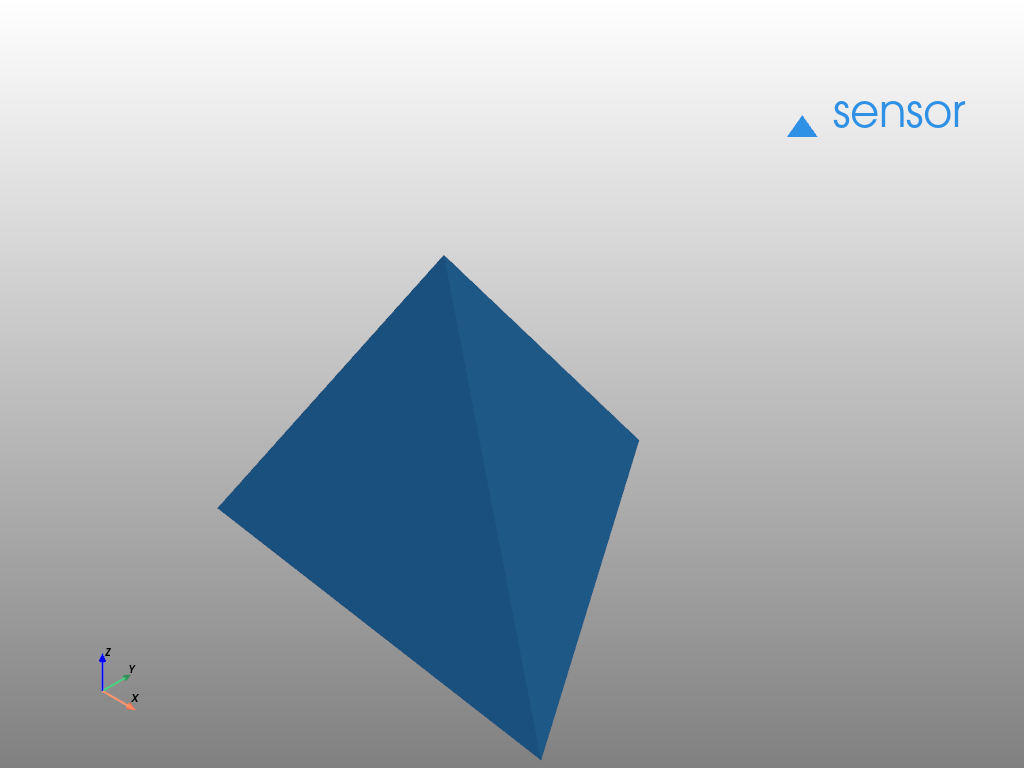
The following example shows how a trace is constructed using the generic backend with the Mesh3d constructor. We create a Sensor object and replace its default 3d model by a tetrahedron.

import magpylib as magpy

# Create trace dictionary
trace_mesh3d = {
    "backend": "generic",
    "constructor": "Mesh3d",
    "kwargs": {
        "x": (1, 0, -1, 0),
        "y": (-0.5, 1.2, -0.5, 0),
        "z": (-0.5, -0.5, -0.5, 1),
        "i": (0, 0, 0, 1),
        "j": (1, 1, 2, 2),
        "k": (2, 3, 3, 3),
        #'opacity': 0.5,
    },
}

# Create sensor
sensor = magpy.Sensor(style_label="sensor")

# Disable default model
sensor.style.model3d.showdefault = False

# Apply custom model
sensor.style.model3d.add_trace(trace_mesh3d)

# Show the system using different backends
for backend in magpy.SUPPORTED_PLOTTING_BACKENDS:
    print(f"Plotting backend: {backend!r}")
    magpy.show(sensor, backend=backend)

Plotting backend: 'matplotlib'

Plotting backend: 'plotly'

Plotting backend: 'pyvista'

/home/docs/checkouts/readthedocs.org/user_builds/magpylib/envs/5.0.3/lib/python3.10/site-packages/pyvista/jupyter/notebook.py:34: UserWarning:

Failed to use notebook backend: 

No module named 'trame'

Falling back to a static output.

As noted above, it is possible to have multiple user-defined traces that will be displayed at the same time. The following example continuation demonstrates this by adding two more traces using the Scatter3d constructor in the generic backend. In addition, it showns how to copy and manipulate Trace3d objects.

# Continuation from above - ensure previous code is executed

import copy
import numpy as np

# Generate trace and add to sensor
ts = np.linspace(0, 2 * np.pi, 30)
trace_scatter3d = {
    "backend": "generic",
    "constructor": "Scatter3d",
    "kwargs": {
        "x": 1.2*np.cos(ts),
        "y": 1.2*np.sin(ts),
        "z": np.zeros(30),
        "mode": "lines",
    },
}
sensor.style.model3d.add_trace(trace_scatter3d)

# Generate new trace from Trace3d object
trace2 = copy.deepcopy(sensor.style.model3d.data[1])
trace2.kwargs["x"] = np.zeros(30)
trace2.kwargs["z"] = 1.2*np.cos(ts)

sensor.style.model3d.add_trace(trace2)

# Show
magpy.show(sensor)

Matplotlib constructors

The following examples show how to construct traces with plot, plot_surface and plot_trisurf:

import matplotlib.pyplot as plt
import matplotlib.tri as mtri
import numpy as np
import magpylib as magpy

# plot trace ###########################

ts = np.linspace(-10, 10, 100)
xs = np.cos(ts) / 100
ys = np.sin(ts) / 100
zs = ts / 20 / 100

trace_plot = {
    "backend": "matplotlib",
    "constructor": "plot",
    "args": (xs, ys, zs),
    "kwargs": {"ls": "--", "lw": 2},
}
magnet = magpy.magnet.Cylinder(polarization=(0, 0, 1), dimension=(0.005, 0.01))
magnet.style.model3d.add_trace(trace_plot)

# plot_surface trace ###################

u, v = np.mgrid[0 : 2 * np.pi : 30j, 0 : np.pi : 20j]
xs = np.cos(u) * np.sin(v) / 100
ys = np.sin(u) * np.sin(v) / 100
zs = np.cos(v) / 100

trace_surf = {
    "backend": "matplotlib",
    "constructor": "plot_surface",
    "args": (xs, ys, zs),
    "kwargs": {"cmap": plt.cm.YlGnBu_r},
}
ball = magpy.Collection(position=(-0.03, 0, 0))
ball.style.model3d.add_trace(trace_surf)

# plot_trisurf trace ###################

u, v = np.mgrid[0 : 2 * np.pi : 50j, -0.5:0.5:10j]
u, v = u.flatten(), v.flatten()

xs = (1 + 0.5 * v * np.cos(u / 2.0)) * np.cos(u) / 100
ys = (1 + 0.5 * v * np.cos(u / 2.0)) * np.sin(u) / 100
zs = 0.5 * v * np.sin(u / 2.0) / 100

tri = mtri.Triangulation(u, v)

trace_trisurf = {
    "backend": "matplotlib",
    "constructor": "plot_trisurf",
    "args": (xs, ys, zs),
    "kwargs": {
        "triangles": tri.triangles,
        "cmap": plt.cm.coolwarm,
    },
}
mobius = magpy.misc.CustomSource(style_model3d_showdefault=False, position=(0.03, 0, 0))
mobius.style.model3d.add_trace(trace_trisurf)

magpy.show(magnet, ball, mobius, backend="matplotlib")

Pre-defined 3D models

Automatic trace generators are provided for several basic 3D models in magpylib.graphics.model3d. They can be used as follows,

from magpylib import Collection
from magpylib.graphics import model3d

# Prism trace ###################################
trace_prism = model3d.make_Prism(
    base=6,
    diameter=2,
    height=1,
    position=(-3, 0, 0),
)
obj0 = Collection(style_label="Prism")
obj0.style.model3d.add_trace(trace_prism)

# Pyramid trace #################################
trace_pyramid = model3d.make_Pyramid(
    base=30,
    diameter=2,
    height=1,
    position=(3, 0, 0),
)
obj1 = Collection(style_label="Pyramid")
obj1.style.model3d.add_trace(trace_pyramid)

# Cuboid trace ##################################
trace_cuboid = model3d.make_Cuboid(
    dimension=(2, 2, 2),
    position=(0, 3, 0),
)
obj2 = Collection(style_label="Cuboid")
obj2.style.model3d.add_trace(trace_cuboid)

# Cylinder segment trace ########################
trace_cylinder_segment = model3d.make_CylinderSegment(
    dimension=(1, 2, 1, 140, 220),
    position=(1, 0, -3),
)
obj3 = Collection(style_label="Cylinder Segment")
obj3.style.model3d.add_trace(trace_cylinder_segment)

# Ellipsoid trace ###############################
trace_ellipsoid = model3d.make_Ellipsoid(
    dimension=(2, 2, 2),
    position=(0, 0, 3),
)
obj4 = Collection(style_label="Ellipsoid")
obj4.style.model3d.add_trace(trace_ellipsoid)

# Arrow trace ###################################
trace_arrow = model3d.make_Arrow(
    base=30,
    diameter=0.6,
    height=2,
    position=(0, -3, 0),
)
obj5 = Collection(style_label="Arrow")
obj5.style.model3d.add_trace(trace_arrow)

obj0.show(obj1, obj2, obj3, obj4, obj5, backend="plotly")

Adding a CAD model

The following code sample shows how a standard CAD model (*.stl file) can be transformed into a Magpylib Trace3d object.

Note

The code below requires installation of the numpy-stl package.

import os
import tempfile

import numpy as np
import requests
from matplotlib.colors import to_hex
from stl import mesh  # requires installation of numpy-stl

import magpylib as magpy


def bin_color_to_hex(x):
    """transform binary rgb into hex color"""
    sb = f"{x:015b}"[::-1]
    r = int(sb[:5], base=2) / 31
    g = int(sb[5:10], base=2) / 31
    b = int(sb[10:15], base=2) / 31
    return to_hex((r, g, b))


def trace_from_stl(stl_file):
    """
    Generates a Magpylib 3D model trace dictionary from an *.stl file.
    backend: 'matplotlib' or 'plotly'
    """
    # Load stl file
    stl_mesh = mesh.Mesh.from_file(stl_file)

    # Extract vertices and triangulation
    p, q, r = stl_mesh.vectors.shape
    vertices, ixr = np.unique(
        stl_mesh.vectors.reshape(p * q, r), return_inverse=True, axis=0
    )
    i = np.take(ixr, [3 * k for k in range(p)])
    j = np.take(ixr, [3 * k + 1 for k in range(p)])
    k = np.take(ixr, [3 * k + 2 for k in range(p)])
    x, y, z = vertices.T

    # Create a generic backend trace
    colors = stl_mesh.attr.flatten()
    facecolor = np.array([bin_color_to_hex(c) for c in colors]).T
    x, y, z = x / 1000, y / 1000, z / 1000  # mm->m
    trace = {
        "backend": "generic",
        "constructor": "mesh3d",
        "kwargs": dict(x=x, y=y, z=z, i=i, j=j, k=k, facecolor=facecolor),
    }
    return trace


# Load stl file from online resource
url = "https://raw.githubusercontent.com/magpylib/magpylib-files/main/PG-SSO-3-2.stl"
file = url.split("/")[-1]
with tempfile.TemporaryDirectory() as temp:
    fn = os.path.join(temp, file)
    with open(fn, "wb") as f:
        response = requests.get(url)
        f.write(response.content)

    # Create traces for both backends
    trace = trace_from_stl(fn)

# Create sensor and add CAD model
sensor = magpy.Sensor(style_label="PG-SSO-3 package")
sensor.style.model3d.add_trace(trace)

# Create magnet and sensor path
magnet = magpy.magnet.Cylinder(polarization=(0, 0, 1), dimension=(0.015, 0.02))
sensor.position = np.linspace((-0.015, 0, 0.008), (-0.015, 0, -0.004), 21)
sensor.rotate_from_angax(np.linspace(0, 180, 21), "z", anchor=0, start=0)

# Display with matplotlib and plotly backends
args = (sensor, magnet)
kwargs = dict(style_path_frames=5)
magpy.show(args, **kwargs, backend="matplotlib")
magpy.show(args, **kwargs, backend="plotly")