Graphic output

3D View

Once all Magpylib objects and their paths have been created, show() creates a 3D plot of the geometric arrangement using the Matplotlib (command line default) and Plotly (notebook default) packages. show() generates a new figure which is automatically displayed.

import magpylib as magpy
import numpy as np

magnet = magpy.magnet.Cylinder(
    polarization=(0, 0, 1),
    dimension=(1, 1),
)
current = magpy.current.Circle(
    current=1,
    diameter=3,
)
dipole = magpy.misc.Dipole(
    moment=(0, 0, 1),
    position=np.linspace((2, 0, -2), (2, 0, 2), 20),
)
sensor = magpy.Sensor(
    pixel=[(0, 0, z) for z in (-0.5, 0, 0.5)],
    position=(-2, 0, 0),
)
magpy.show(magnet, current, dipole, sensor)

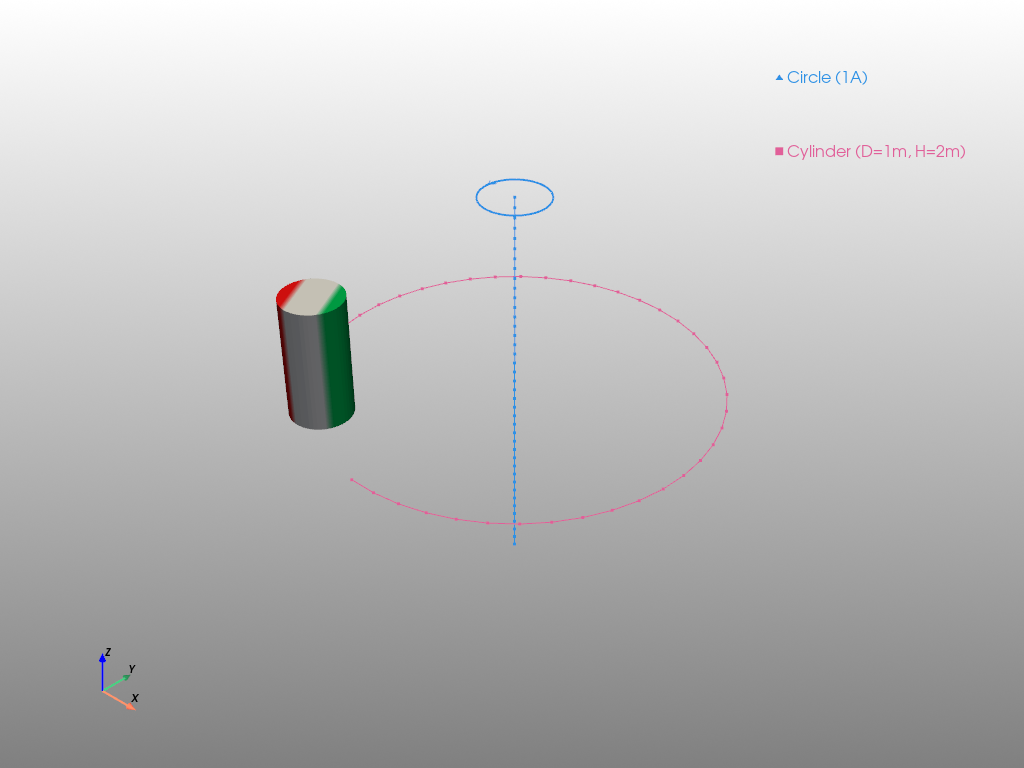
Notice that objects and their paths are automatically assigned different colors. The polarization of the magnet is displayed by default (Plotly and Pyvista) by coloring the poles, which overwrites the object color. In Matplotlib the polarization is by default displayed by an arrow. Current directions and dipole objects are indicated by arrows and sensors are shown as tri-colored coordinate cross with pixel as markers.

How objects are represented graphically (color, line thickness, etc.) is defined by their style properties.

---

Graphic Backends

The graphic backend refers to the plotting library that is used for graphic output. A plotting canvas refers to the frame/window/canvas/axes object the graphic output is forwarded to.

The graphic backend is set via the kwarg backend in the show() function, which is demonstrated in the following example

import magpylib as magpy
import numpy as np

# Define sources and paths
loop = magpy.current.Circle(
    current=1, diameter=1, position=np.linspace((0, 0, -3), (0, 0, 3), 40)
)
cylinder = magpy.magnet.Cylinder(
    polarization=(0, -1, 0), dimension=(1, 2), position=(0, -3, 0)
)
cylinder.rotate_from_angax(np.linspace(0, 300, 40), "z", anchor=0, start=0)

for backend in magpy.SUPPORTED_PLOTTING_BACKENDS:
    print(backend)
    magpy.show(loop, cylinder, backend=backend)

matplotlib

plotly

pyvista

2026-06-02 06:44:40.400 (   4.213s) [    7B168792FB80]vtkXOpenGLRenderWindow.:1460  WARN| bad X server connection. DISPLAY=
/home/docs/checkouts/readthedocs.org/user_builds/magpylib/checkouts/latest/src/magpylib/_src/display/backend_pyvista.py:366: UserWarning:

Using static image for notebook display.
Install trame for interactive backends: pip install "pyvista[jupyter]"

With the installation default setting, backend='auto', Magpylib infers the graphic backend from the environment running the code, or from the requested canvas.

environment	canvas	inferred backend
Command-Line	None	matplotlib
IPython notebook	None	plotly
all	matplotlib.axes.Axes	matplotlib
all	plotly.graph_objects.Figure or FigureWidget	plotly
all	pyvista.Plotter	pyvista

The library default can be changed, e.g. with the command magpy.defaults.display.backend = 'plotly'.

There is a high level of feature parity, however, not all graphic features are supported by all backends, and not all graphic features work equally well, so that default style settings differ slightly. In addition, some common Matplotlib syntax (e.g. color 'r', linestyle ':') is automatically translated to other backends.

Feature	Matplotlib	Plotly	Pyvista
triangular mesh 3d	✔️	✔️	✔️
line 3d	✔️	✔️	✔️
line style	✔️	✔️	❌
line color	✔️	✔️	✔️
line width	✔️	✔️	✔️
marker 3d	✔️	✔️	✔️
marker color	✔️	✔️	✔️
marker size	✔️	✔️	✔️
marker symbol	✔️	✔️	❌
marker numbering	✔️	✔️	❌
zoom level	✔️	✔️	❌[2]
magnetization color	✔️[7]	✔️	✔️
animation	✔️	✔️	✔️[5]
animation time	✔️	✔️	✔️[5]
animation fps	✔️	✔️	✔️[5]
animation slider	✔️[1]	✔️	❌
subplots 2D	✔️	✔️	✔️[6]
subplots 3D	✔️	✔️	✔️
user canvas	✔️	✔️	✔️
user extra 3d model [3]	✔️	✔️	✔️[4]

[1]: when returning animation object and exporting it as jshtml.

[2]: possible but not implemented at the moment.

[3]: only 'scatter3d', and 'mesh3d'. Gets “translated” to every other backend.

[4]: custom user defined trace constructors allowed, which are specific to the backend.

[5]: animation is only available through export as gif or mp4

[6]: 2D plots are not supported for all jupyter_backends. As of pyvista>=0.38 these are deprecated and replaced by the trame backend.

[7]: Matplotlib does not support color gradient. Instead magnetization is shown through object slicing and coloring.

show() will also pass on all kwargs to the respective plotting backends. For example, in the animation sample code the kwarg show_legend is forwarded to the Plotly backend.

---

Plotting Canvas

When calling show(), a figure is automatically generated and displayed. It is also possible to place the show() output in a given figure using the canvas argument. Consider the following Magpylib field computation,

import magpylib as magpy
import numpy as np

# Magpylib field computation
loop = magpy.current.Circle(current=1, diameter=0.1)
sens = magpy.Sensor(position=np.linspace((0, 0, -0.1), (0, 0, 0.1), 100))
B = loop.getB(sens)

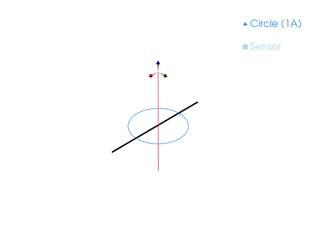
The following examples demonstrate how to place the Magpylib show() output in figures created with the three supported graphic backends.

In Matplotlib we combine a 2D-field plot with the 3D show output and modify the 3D show output with a line.

import magpylib as magpy
import matplotlib.pyplot as plt
import numpy as np

# Magpylib field computation
loop = magpy.current.Circle(current=1, diameter=0.1)
sens = magpy.Sensor(position=np.linspace((0, 0, -0.1), (0, 0, 0.1), 100))
B = loop.getB(sens)

# Create Matplotlib figure with subplots
fig = plt.figure(figsize=(10, 4))
ax1 = fig.add_subplot(121)
ax2 = fig.add_subplot(122, projection="3d")

# 2D Matplotlib plot
ax1.plot(B)

# Place Magpylib show output in Matplotlib figure
magpy.show(loop, sens, canvas=ax2)

# Modify show output
ax2.plot([-0.1, 0.1], [0, 0], [0, 0], color="k")

# Render figure
plt.tight_layout()
plt.show()

Attention

When providing a canvas, no update to its layout is performed by Magpylib, unless explicitly specified by setting canvas_update=True in show(). By default canvas_update='auto' only updates the canvas if is not provided by the user. The example above outputs a 3D scene with the default Matplotlib settings and will not match the standard Magpylib settings.

In Plotly we combine a 2D-field plot with the 3D show output and modify the 3D show output with a line.

import magpylib as magpy
import numpy as np
import plotly.graph_objects as go

# Magpylib field computation
loop = magpy.current.Circle(current=1, diameter=0.1)
sens = magpy.Sensor(position=np.linspace((0, 0, -0.1), (0, 0, 0.1), 100))
B = loop.getB(sens)

# Create Plotly figure and subplots
fig = go.Figure().set_subplots(
    rows=1, cols=2, specs=[[{"type": "xy"}, {"type": "scene"}]]
)

# 2D Plotly plot
fig.add_scatter(y=B[:, 2], name="Bz")

# Draw 3d model in the existing Plotly figure
magpy.show(loop, sens, canvas=fig, col=2, canvas_update=True)

# Add 3d scatter trace to main figure model
fig.add_scatter3d(x=(-0.1, 0.1), y=(0, 0), z=(0, 0), col=2, row=1)

# Render figure
fig.show()

Pyvista is not made for 2D plotting. Here we simply add a line to the 3D show output.

# Continuation from above - ensure previous code is executed

import pyvista as pv

# Create Pyvista scene
pl = pv.Plotter()

# Place Magpylib show output in Pyvista scene
magpy.show(loop, sens, canvas=pl)

# Add a Line to 3D scene
line = np.array([(-0.1, 0, 0), (0.1, 0, 0)])
pl.add_lines(line, color="black")

# Render figure
pl.show()

/tmp/ipykernel_1456/1414728667.py:16: UserWarning:

Using static image for notebook display.
Install trame for interactive backends: pip install "pyvista[jupyter]"

---

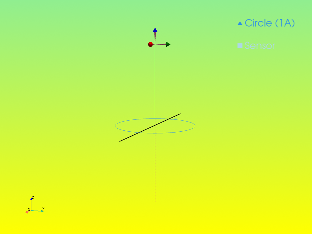
Return Figure

Instead of forwarding a figure to an existing canvas, it is also possible to return the figure object for further manipulation using the return_fig command. In the following example this is demonstrated for the pyvista backend.

import magpylib as magpy
import numpy as np

# Create Magpylib objects with paths
loop = magpy.current.Circle(current=1, diameter=0.1)
sens = magpy.Sensor(position=np.linspace((0, 0, -0.1), (0, 0, 0.1), 100))

# Return pyvista scene object with show
pl = magpy.show(loop, sens, backend="pyvista", return_fig=True)

# Modify Pyvista scene
pl.add_lines(np.array([(-0.1, 0, 0), (0.1, 0, 0)]), color="black")
pl.camera.position = (0.5, 0.2, 0.1)
pl.set_background("yellow", top="lightgreen")
pl.enable_anti_aliasing("ssaa")

# Display scene
pl.show()

/tmp/ipykernel_1456/3604688952.py:18: UserWarning:

Using static image for notebook display.
Install trame for interactive backends: pip install "pyvista[jupyter]"

---

Animation

The Magpylib object paths visualized with show() can be animated by setting the kwarg animation=True. This synergize specifically well with the Plotly backend.

The animations can be fine-tuned with the following kwargs of show():

1. animation_time (default=3), must be a positive number that gives the animation time in seconds.

2. animation_slider (default=True), is boolean and sets if a slider should be displayed.

3. animation_fps (default=30), sets the maximal frames per second.

Each path step will generate one frame of the animation, unless animation_fps would be exceeded. In this case specific equidistant frames will be selected automatically to adjust to the limited display possibilities. For practicality, the input animation=x will automatically set animation=True and animation_time=x.

The following example demonstrates the animation feature,

import magpylib as magpy
import numpy as np

# Create Magpylib objects with paths
loop = magpy.current.Circle(current=1, diameter=0.1)
sens = magpy.Sensor(position=np.linspace((0, 0, -0.1), (0, 0, 0.1), 100))

# Show animation
magpy.show(
    loop,
    sens,
    animation=1,
    animation_fps=20,
    animation_slider=True,
    backend="plotly",
    showlegend=False,
)

Warning

Even with some implemented fail safes, such as a maximum frame rate and frame count, there is no guarantee that the animation will be rendered properly. This is particularly relevant when the user tries to animate many objects and/or many path positions at the same time.

---

Built-in Subplots

Added in version 4.4: Coupled subplots

It is often tedious to integrate the Magpylib show() output into sub-plots as shown above, especially when dealing with animations and combinations of 2D and 3D plots.

For this, Magpylib offers the possibility to show the sensor output along a path in addition to the 3D-output, and to place 2D and 3D outputs in subplots.

With show

All of this is achieved via the show() function by passing input objects as dictionaries with the arguments.

1. objects: list of Magpylib objects

2. col: int which selects the subplot column. Default is col=1.

3. row: int which selects the subplot row. Default is row=1.

4. output: string which selects the type of output that should be displayed in this subplot. Options are

   1. 'model3d' is the default value and selects the 3D output.

   2. 'Xa' selects a 2D line-plot of a field component (combination) as seen by the sensor(s) along their path. The sensor(s) must be part of the objects input. Here “X” selects the field and must be one of “BHJM”, and “a” selects the respective component combination and must be a subset of “xyz”. For example, output=Hx displays the x-component of the H-field, or output=Bxz displays sqrt(|Bx|² + |Bz|²). By default, source outputs are summed up (sumup=True) and sensor pixels, are aggregated by mean (pixel_agg='mean').

The following code demonstrates these features.

import magpylib as magpy
import numpy as np

# Create Magpylib objects with paths
loop = magpy.current.Circle(current=1, diameter=0.1, style_label="L")
sens = magpy.Sensor(
    position=np.linspace((-0.1, 0, 0.1), (0.1, 0, 0.1), 50), style_label="S"
)

# Use built-in subplots
magpy.show(
    {"objects": [loop, sens]},
    {"objects": [loop, sens], "output": "Bx", "col": 2},
    {"objects": [loop, sens], "output": ["Hx", "Hy", "Hz"], "row": 2},
    {"objects": [loop, sens], "output": "Hxyz", "col": 2, "row": 2},
    backend="matplotlib",
)

Each input dictionary can contain kwargs, like pixel_agg=None or sumup=False for 2D plots.

import magpylib as magpy
import numpy as np

# Create Magpylib objects with paths
loop1 = magpy.current.Circle(current=1, diameter=0.1, style_label="L1")
loop2 = loop1.copy(diameter=0.2, style_label="L2")
sens = magpy.Sensor(
    pixel=[(0.01, 0, 0), (-0.01, 0, 0)],
    position=np.linspace((-0.2, 0, 0.1), (0.2, 0, 0.1), 50),
    style_label="S",
)
obj = [loop1, loop2, sens]

# Use built-in subplots
magpy.show(
    {"objects": obj, "output": "Hx"},
    {"objects": obj, "output": "Hx", "pixel_agg": None, "col": 2},
    {"objects": obj, "output": "Hx", "sumup": False, "row": 2},
    {
        "objects": obj,
        "output": "Hx",
        "pixel_agg": None,
        "sumup": False,
        "row": 2,
        "col": 2,
    },
)

With show_context

To make the subplot syntax more convenient we introduced the show_context native Python context manager. It allows to defer calls to the show() function while passing additional arguments. This is necessary for Magpylib to know how many rows and columns are requested by the user, which single show() calls do not keep track of. All kwargs, e.g. backend are handed directly to the context manager.

The above example becomes:

import magpylib as magpy
import numpy as np

# Create Magpylib objects with paths
loop = magpy.current.Circle(current=1, diameter=0.1, style_label="L")
sens = magpy.Sensor(
    position=np.linspace((-0.1, 0, 0.1), (0.1, 0, 0.1), 50), style_label="S"
)

# Use built-in subplots via show_context
with magpy.show_context(loop, sens, backend="plotly") as sc:
    sc.show()
    sc.show(output="Bx", col=2)
    sc.show(output=["Hx", "Hy", "Hz"], row=2)
    sc.show(output="Hxyz", col=2, row=2)

Note

Using the context manager object as in:

import magpylib as magpy

obj1 = magpy.magnet.Cuboid()
obj2 = magpy.magnet.Cylinder()

with magpy.show_context() as sc:
    sc.show(obj1, col=1)
    sc.show(obj2, col=2)

is equivalent to the use of magpylib.show directly, as long as within the context manager:

import magpylib as magpy

obj1 = magpy.magnet.Cuboid()
obj2 = magpy.magnet.Cylinder()

with magpy.show_context():
    magpy.show(obj1, col=1)
    magpy.show(obj2, col=2)

Coupled 2D/3D Animation

It is very helpful to combine 2D and 3D subplots in an animation that shows the motion of the 3D system, while displaying the field at the respective path instance at the same time. Unfortunately, it is quite tedious to create such animations. The most powerful feature and main reason behind built-in subplots is the ability to do just that with few lines of code.

import magpylib as magpy
import numpy as np

# Create Magpylib objects with paths
loop = magpy.current.Circle(current=1, diameter=0.1, style_label="L")
sens = magpy.Sensor(
    position=np.linspace((-0.1, 0, 0.1), (0.1, 0, 0.1), 50), style_label="S"
)

# Use built-in subplots via show_context
with magpy.show_context(loop, sens, animation=True) as sc:
    sc.show()
    sc.show(output="Bx", col=2)
    sc.show(output=["Hx", "Hy", "Hz"], row=2)
    sc.show(output="Hxyz", col=2, row=2)

Canvas Length Units

When displaying very small Magpylib objects, the axes scaling in units (m) might be inadequate and you may want to use other units that fit the system dimensions more nicely. The example below shows how to display an object (in this case the same) with different length units and zoom levels.

Tip

Setting units_length='auto' will infer the most suitable units based on the maximum range of the system.

import magpylib as magpy

c1 = magpy.magnet.Cuboid(dimension=(0.001, 0.001, 0.001), polarization=(1, 2, 3))

with magpy.show_context(c1, backend="matplotlib") as s:
    s.show(row=1, col=1, units_length="auto", zoom=0)
    s.show(row=1, col=2, units_length="mm", zoom=1)
    s.show(row=2, col=1, units_length="µm", zoom=2)
    s.show(row=2, col=2, units_length="m", zoom=3)