Floating Magnets#

Magpylib’s efficient field and force computations make it ideal for dynamic simulations that require solving equations of motion through time-discretization methods. This example demonstrates how to implement numerical integration schemes to simulate the motion of magnetic objects under electromagnetic forces and torques.

Mathematical Formalism#

The dynamics of magnetic objects are governed by the classical equations of motion: \(\vec{F} = \dot{\vec{p}}\) for translation (with force \(\vec{F}\) and momentum \(\vec{p}\)) and \(\vec{T} = \dot{\vec{L}}\) for rotation (with torque \(\vec{T}\) and angular momentum \(\vec{L}\)).

For numerical integration, we implement a first-order semi-implicit Euler method—a robust algorithm commonly used for planetary motion and other dynamic systems. This method discretizes time into small steps \(\Delta t\) and updates the system state sequentially.

Translation dynamics: For position \(\vec{s}\), velocity \(\vec{v} = \dot{\vec{s}}\), and mass \(m\):

\[\vec{v}(t+\Delta t) = \vec{v}(t) + \frac{\Delta t}{m} \vec{F}(t)\]

\[\vec{s}(t+\Delta t) = \vec{s}(t) + \Delta t \cdot \vec{v} (t + \Delta t)\]

Rotational dynamics: For orientation angle \(\vec{\varphi}\), angular velocity \(\vec{\omega}\), and inertia tensor \(J\):

\[\vec{\omega} (t + \Delta t) = \vec{ω}(t) + \Delta t \cdot J^{-1} \cdot \vec{T}(t)\]

\[\vec{\varphi} (t + \Delta t) = \vec{\varphi}(t) + \Delta t \cdot \vec{\omega} (t + \Delta t) \]

The semi-implicit nature (velocity updated before position) provides better numerical stability compared to explicit methods, making it well-suited for magnetic dynamics where forces can vary rapidly with distance.

Magnet Accelerated by Coil#

This implementation demonstrates the proposed Euler scheme using a simplified scenario where cubical magnets are accelerated along the z-axis by a current loop, as shown in the following sketch:

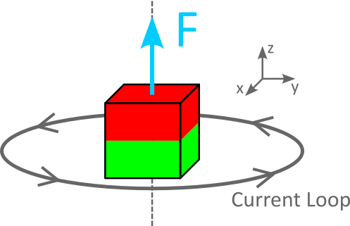
Sketch of current loop and magnet. — A cubical magnet is accelerated by a current loop.#

Due to the axial symmetry of this configuration, the net torque on the magnet is zero, allowing us to solve only the translational equations of motion while ignoring rotational dynamics.

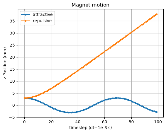
The simulation starts with two magnets (opposite magnetization) at rest, positioned slightly above the current loop center along the z-axis. As time progresses, magnetic forces accelerate the magnets, and their z-positions are computed and visualized to demonstrate the different behaviors based on magnetic moment orientation.

../../../_images/62db44550828fd9a189cd7725086e27a0ffa188448292bb1587054a75c2205de.png

Key observations:

The simulation compares two magnets with opposite polarizations. In the repulsive case (orange), the magnetic moments of the magnet and coil are antiparallel, causing the magnet to be pushed away from the coil in the positive z-direction with monotonic acceleration. In the attractive case (blue), the moments are parallel, initially accelerating the magnet toward the coil center. Due to inertia, the magnet overshoots and emerges on the opposite side, where it is again attracted back toward the center, resulting in oscillatory motion around the equilibrium position.

Warning

This numerical algorithm accumulates discretization errors over time. For higher accuracy or longer simulations, use smaller timesteps or higher-order integration methods.

Two-Body Problem#

In the following example we demonstrate a fully dynamic simulation with two magnetic bodies that rotate around each other, attracted towards each other by the magnetic force, and repelled by the centrifugal force.

Sketch of two-magnet ringdown. — Two freely moving magnets rotate around each other.#

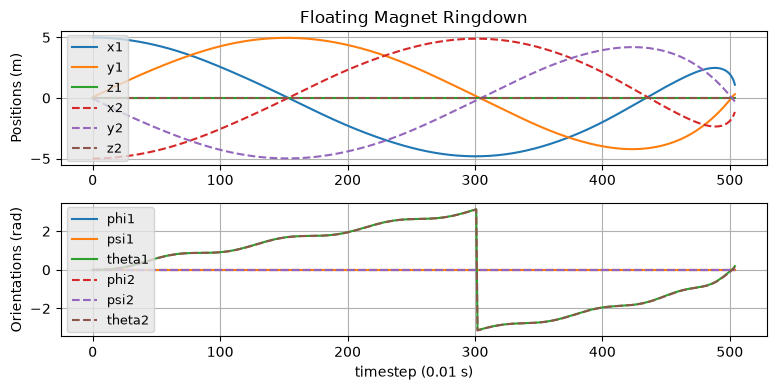
Contrary to the simple case above, we apply the Euler scheme also to the rotation degrees of freedom, as the magnets will change their orientation while they circle around each other. Magnet positions and orientations are computed and visualized.

Show code cell source

Hide code cell source

import numpy as np
import matplotlib.pyplot as plt
import magpylib as magpy
from scipy.spatial.transform import Rotation as R

def timestep(source, target, dt):
    """
    Apply full Euler-sceme timestep to target.

    Parameters:
    -----------
    source: Magpylib source object that generates the magnetic field

    target: Magpylib target object viable for force computation. In addition,
        the target object must have the following parameters describing
        the motion state: v (velocity), m (mass), w (angular velocity),
        I_inv (inverse inertial tensor)

    dt: Euler scheme length of timestep
    """
    # Compute force
    F, T = magpy.getFT(source, target)

    # Set new velocity and position
    target.v = target.v + dt/target.m * F
    target.position = target.position + dt * target.v

    # Set new angular velocity and rotation angle
    target.w = target.w + dt*target.orientation.apply(np.dot(target.I_inv, target.orientation.inv().apply(T)))
    target.orientation = R.from_rotvec(dt*target.w)*target.orientation

# Simulation parameters
steps=505   # number of timesteps
dt = 1e-2   # timstep size (s)

# Initial conditions
pos0a, pos0b = (5, 0, 0), (-5, 0, 0)  # m
v0 = np.array((0, 5.18, 0))       # m/s
m0 = 2                            # kg
w0 = np.array([0, 0, 0])          # rad/s
I0 = 1 * np.eye(3)                # kg*m²

# Create the two magnets and set initial conditions
sphere1 = magpy.magnet.Sphere(position=pos0a, diameter=1, polarization=(1, 0, 0))
sphere1.m = m0
sphere1.v = v0
sphere1.w = w0
sphere1.I_inv = I0

sphere2 = sphere1.copy(position=pos0b)
sphere2.v = -v0

# Solve equations of motion
data = np.zeros((4, steps, 3))
for i in range(steps):
    timestep(sphere1, sphere2, dt)
    timestep(sphere2, sphere1, dt)

    # Store results of each timestep
    data[0,i] = sphere1.position
    data[1,i] = sphere2.position
    data[2,i] = sphere1.orientation.as_euler('xyz')
    data[3,i] = sphere2.orientation.as_euler('xyz')

# Plot results
fig, (ax1,ax2) = plt.subplots(2, 1, figsize=(8, 4))

for j,ls in enumerate(["-", "--"]):

    # Plot positions
    for i,a in enumerate("xyz"):
        ax1.plot(data[j,:,i], label= a + str(j+1), ls=ls)

    # Plot orientations
    for i,a in enumerate(["phi", "psi", "theta"]):
        ax2.plot(data[j+2,:,i], label= a + str(j+1), ls=ls)

# Figure styling
for ax in fig.axes:
    ax.legend(fontsize=9, loc=6, facecolor='.9')
    ax.grid()
ax1.set(
    title="Floating Magnet Ringdown",
    ylabel="Positions (m)",
)
ax2.set(
    ylabel="Orientations (rad)",
    xlabel="timestep (0.01 s)",
)
plt.tight_layout()
plt.show()

../../../_images/f761f4b0e090b614fdffe9a7a491794391ccde579ea48d835b11a6f08fb22fb9.png

Key observations:

In the figure one can see, that the initial velocity is chosen so that the magnets approach each other in a ringdown-like behavior. The magnets are magnetically locked towards each other - both always show the same orientation. However, given no initial angular velocity, the rotation angle is oscillating several times while circling once.

A video is helpful in this case to understand what is going on. From the computation above, we build the following gif making use of this export-animation tutorial.

animation of simulated magnet ringdown. — Animation of above simulated magnet ringdown.#

Note

Keep in mind that this simulation accounts only for magnetic forces. Time dependent magnetic fields induce eddy currents in conductive media which are not considered here.