Graphics

Once all Magpylib objects and their paths have been created, show provides a convenient way to graphically display the geometric arrangement using the Matplotlib (default) and Plotly packages. When show is called, it generates a new figure which is then automatically displayed.

The desired graphic backend is selected with the backend keyword argument. To bring the output to a given, user-defined figure, the canvas argument is used. This is demonstrated in Plotting backends.

The following example shows the graphical representation of various Magpylib objects and their paths using the default Matplotlib graphic backend.

import numpy as np
import pyvista as pv

import magpylib as magpy

objects = {
    "Cuboid": magpy.magnet.Cuboid(
        polarization=(0, -0.1, 0),
        dimension=(0.01, 0.01, 0.01),
        position=(-0.06, 0, 0),
    ),
    "Cylinder": magpy.magnet.Cylinder(
        polarization=(0, 0, 0.01),
        dimension=(0.01, 0.01),
        position=(-0.05, 0, 0),
    ),
    "CylinderSegment": magpy.magnet.CylinderSegment(
        polarization=(0, 0, 0.01),
        dimension=(0.003, 0.01, 0.01, 0, 140),
        position=(-0.03, 0, 0),
    ),
    "Sphere": magpy.magnet.Sphere(
        polarization=(0, 0, 0.01),
        diameter=0.01,
        position=(-0.01, 0, 0),
    ),
    "Tetrahedron": magpy.magnet.Tetrahedron(
        polarization=(0, 0, 0.01),
        vertices=((-0.01, 0, 0), (0.01, 0, 0), (0, -0.01, 0), (0, -0.01, -0.01)),
        position=(-0.04, 0, 0.04),
    ),
    "TriangularMesh": magpy.magnet.TriangularMesh.from_pyvista(
        polarization=(0, 0, 0.01),
        polydata=pv.Dodecahedron(radius=0.01),
        position=(-0.01, 0, 0.04),
    ),
    "Circle": magpy.current.Circle(
        current=1,
        diameter=0.01,
        position=(0.04, 0, 0),
    ),
    "Polyline": magpy.current.Polyline(
        current=1,
        vertices=[
            (0.01, 0, 0),
            (0, 0.01, 0),
            (-0.01, 0, 0),
            (0, -0.01, 0),
            (0.01, 0, 0),
        ],
        position=(0.01, 0, 0),
    ),
    "Dipole": magpy.misc.Dipole(
        moment=(0, 0, 1),
        position=(0.03, 0, 0),
    ),
    "Triangle": magpy.misc.Triangle(
        polarization=(0, 0, 0.01),
        vertices=((-0.01, 0, 0), (0.01, 0, 0), (0, 0.01, 0)),
        position=(0.02, 0, 0.04),
    ),
    "Sensor": magpy.Sensor(
        pixel=[(0, 0, z) for z in (-0.005, 0, 0.005)],
        position=(0, -0.03, 0),
    ),
}

objects["Circle"].move(np.linspace((0, 0, 0), (0, 0, 0.05), 20))
objects["Cuboid"].rotate_from_angax(np.linspace(0, 90, 20), "z", anchor=0)

magpy.show(*objects.values())

Notice that objects and their paths are automatically assigned different colors, the magnetization is shown by coloring the poles (default) or by an arrow (via styles). Current directions and dipole objects are indicated by arrows and sensors are shown as tri-colored coordinate cross with pixel as markers.

How objects are represented graphically (color, line thickness, etc.) is defined by their style properties. The default style, which can be seen above, is accessed and manipulated through magpy.defaults.display.style. In addition, each object can have an individual style, which takes precedence over the default setting. A local style override is also possible by passing style arguments directly to show.

The hierarchy that decides about the final graphic object representation, a list of all style parameters and other options for tuning the show-output are described in Styles and Animation.

Plotting backends

The plotting backend refers to the plotting library that is used for graphic output. Canvas refers to the frame/window/canvas/axes object the graphic output is forwarded to.

Magpylib supports several common graphic backends.

from magpylib import SUPPORTED_PLOTTING_BACKENDS

SUPPORTED_PLOTTING_BACKENDS

('matplotlib', 'plotly', 'pyvista')

The installation default is set to 'auto'. In this case the backend is dynamically inferred depending on the current running environment (command-line or notebook), the available installed backend libraries and the set canvas:

environment	canvas	inferred backend
Command-Line	None	matplotlib
IPython notebook	None	plotly if installed else matplotlib
all	matplotlib.axes.Axes	matplotlib
all	plotly.graph_objects.Figure (or FigureWidget)	plotly
all	pyvista.Plotter	pyvista

To explicitly select a graphic backend one can

1. Change the library default with magpy.defaults.display.backend = 'plotly'.

2. Set the backend kwarg in the show function, show(..., backend='matplotlib').

There is a high level of feature parity, however, not all graphic features are supported by all backends. In addition, some common Matplotlib syntax (e.g. color 'r', linestyle ':') is automatically translated to other backends.

Feature	Matplotlib	Plotly	Pyvista
triangular mesh 3d	✔️	✔️	✔️
line 3d	✔️	✔️	✔️
line style	✔️	✔️	❌
line color	✔️	✔️	✔️
line width	✔️	✔️	✔️
marker 3d	✔️	✔️	✔️
marker color	✔️	✔️	✔️
marker size	✔️	✔️	✔️
marker symbol	✔️	✔️	❌
marker numbering	✔️	✔️	❌
zoom level	✔️	✔️	❌[2]
magnetization color	✔️[7]	✔️	✔️
animation	✔️	✔️	✔️[5]
animation time	✔️	✔️	✔️[5]
animation fps	✔️	✔️	✔️[5]
animation slider	✔️[1]	✔️	❌
subplots 2D	✔️	✔️	✔️[6]
subplots 3D	✔️	✔️	✔️
user canvas	✔️	✔️	✔️
user extra 3d model [3]	✔️	✔️	✔️ [4]

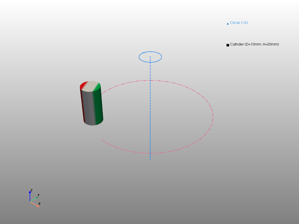
The following example demonstrates the currently supported backends:

import numpy as np
import pyvista as pv

import magpylib as magpy

# define sources and paths
loop = magpy.current.Circle(current=1, diameter=0.01)
loop.position = np.linspace((0, 0, -3), (0, 0, 3), 40) / 100

cylinder = magpy.magnet.Cylinder(
    polarization=(0, -0.1, 0), dimension=(0.01, 0.02), position=(0, -0.03, 0)
)
cylinder.rotate_from_angax(np.linspace(0, 300, 40), "z", anchor=0, start=0)

# show the system using different backends
for backend in magpy.SUPPORTED_PLOTTING_BACKENDS:
    print(f"Plotting backend: {backend!r}")
    magpy.show(loop, cylinder, backend=backend)

Plotting backend: 'matplotlib'

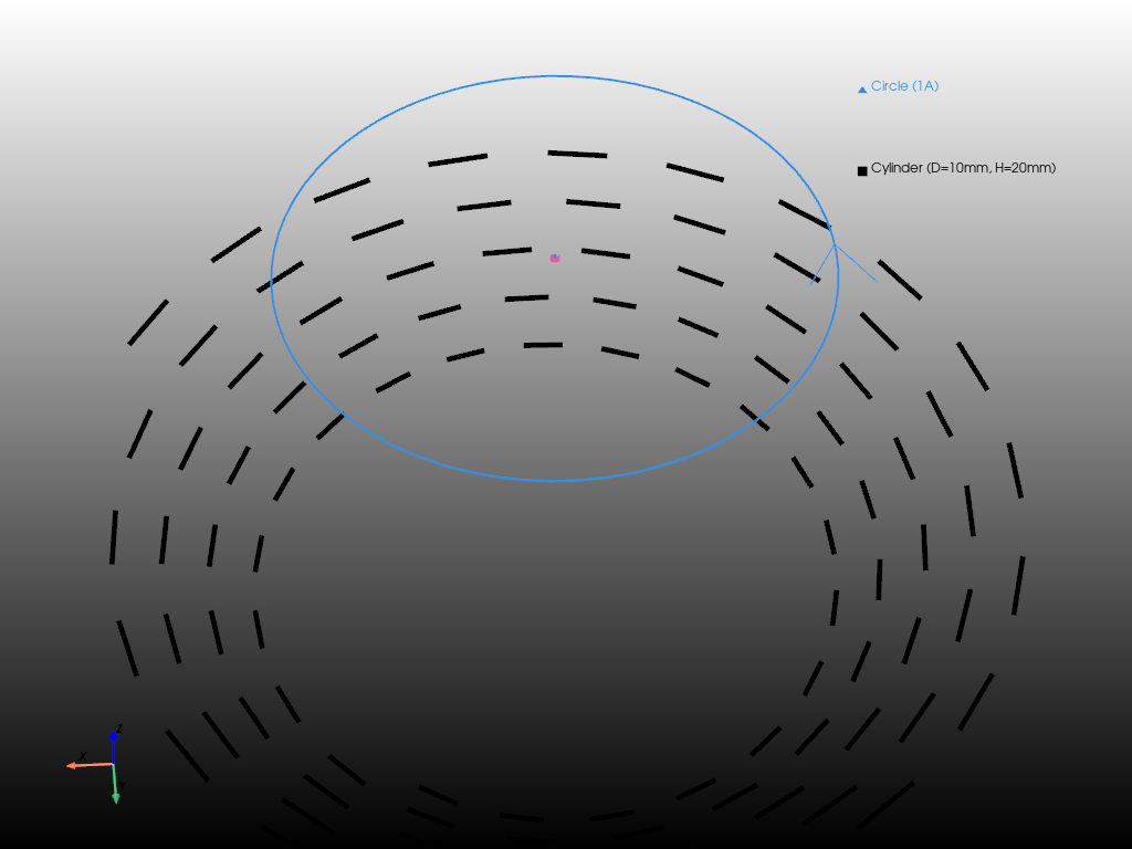
Plotting backend: 'plotly'

Plotting backend: 'pyvista'

/home/docs/checkouts/readthedocs.org/user_builds/magpylib/envs/stable/lib/python3.9/site-packages/pyvista/jupyter/notebook.py:34: UserWarning:

Failed to use notebook backend: 

No module named 'trame'

Falling back to a static output.

Output in custom figure

When calling show, a figure is automatically generated and displayed. It is also possible to display the show output on a given user-defined canvas with the canvas argument.

In the following example we show how to combine a 2D field plot with the 3D show output in Matplotlib:

import matplotlib.pyplot as plt
import numpy as np

import magpylib as magpy

# setup matplotlib figure and subplots
fig = plt.figure(figsize=(10, 4))
ax1 = fig.add_subplot(121)  # 2D-axis
ax2 = fig.add_subplot(122, projection="3d")  # 3D-axis

# define sources and paths
loop = magpy.current.Circle(current=1, diameter=0.01)
loop.position = np.linspace((0, 0, -3), (0, 0, 3), 40) / 100

cylinder = magpy.magnet.Cylinder(
    polarization=(0, -0.1, 0), dimension=(0.01, 0.02), position=(0, -0.03, 0)
)
cylinder.rotate_from_angax(np.linspace(0, 300, 40)[1:], "z", anchor=0)

# compute field and plot in 2D-axis
B = magpy.getB([loop, cylinder], (0, 0, 0), sumup=True)
ax1.plot(B)

# display show() output in 3D-axis
magpy.show(loop, cylinder, canvas=ax2)

# generate figure
plt.tight_layout()
plt.show()

A similar example with Plotly:

import numpy as np
import plotly.graph_objects as go

import magpylib as magpy

# setup plotly figure and subplots
fig = go.Figure().set_subplots(
    rows=1, cols=2, specs=[[{"type": "xy"}, {"type": "scene"}]]
)

# define sources and paths
loop = magpy.current.Circle(current=1, diameter=0.01)
loop.position = np.linspace((0, 0, -3), (0, 0, 3), 40) / 100

cylinder = magpy.magnet.Cylinder(
    polarization=(0, -0.1, 0), dimension=(0.01, 0.02), position=(0, -0.03, 0)
)
cylinder.rotate_from_angax(np.linspace(0, 300, 40)[1:], "z", anchor=0)

# compute field and plot in 2D-axis
B = magpy.getB([loop, cylinder], (0, 0, 0), sumup=True)
for i, lab in enumerate(["Bx", "By", "Bz"]):
    fig.add_trace(go.Scatter(x=np.linspace(0, 1, 40), y=B[:, i], name=lab))

# display show() output in 3D-axis
temp_fig = go.Figure()
magpy.show(loop, cylinder, canvas=temp_fig, backend="plotly")
fig.add_traces(temp_fig.data, rows=1, cols=2)
fig.layout.scene.update(temp_fig.layout.scene)

# generate figure
fig.show()

An example with Pyvista:

import numpy as np
import pyvista as pv

import magpylib as magpy

# define sources and paths
loop = magpy.current.Circle(current=1, diameter=5)
loop.position = np.linspace((0, 0, -3), (0, 0, 3), 40) / 100

cylinder = magpy.magnet.Cylinder(
    polarization=(0, -0.1, 0), dimension=(0.01, 0.02), position=(0, -0.03, 0)
)
cylinder.rotate_from_angax(np.linspace(0, 300, 40)[1:], "z", anchor=0)

# create a pyvista plotting scene with some graphs
pl = pv.Plotter()
line = np.array(
    [(t * np.cos(15 * t), t * np.sin(15 * t), t - 8) for t in np.linspace(3, 5, 200)]
)
pl.add_lines(line, color="black")

# add magpylib.show() output to existing scene
magpy.show(loop, cylinder, backend="pyvista", canvas=pl)

# display scene
pl.camera.position = (.50, 10, 10)
pl.set_background("black", top="white")
pl.show()

/home/docs/checkouts/readthedocs.org/user_builds/magpylib/envs/stable/lib/python3.9/site-packages/pyvista/jupyter/notebook.py:34: UserWarning:

Failed to use notebook backend: 

No module named 'trame'

Falling back to a static output.

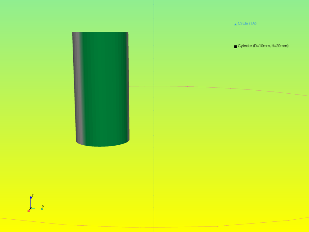
Return figure

Instead of forwarding a figure to an existing canvas, it is also possible to return the figure object for further manipulation using the return_fig command. In the following example this is demonstrated for the pyvista backend.

import numpy as np
import pyvista as pv

import magpylib as magpy

# define sources and paths
loop = magpy.current.Circle(current=1, diameter=0.05)
loop.position = np.linspace((0, 0, -3), (0, 0, 3), 40) / 100

cylinder = magpy.magnet.Cylinder(
    polarization=(0, -0.1, 0), dimension=(0.01, 0.02), position=(0, -0.03, 0)
)
cylinder.rotate_from_angax(np.linspace(0, 300, 40)[1:], "z", anchor=0)

# return pyvista scene from magpylib.show()
pl = magpy.show(loop, cylinder, backend="pyvista", return_fig=True)

# add line to the pyvista scene
line = np.array(
    [
        (t * np.cos(15 * t), t * np.sin(15 * t), t - 8)
        for t in np.linspace(0.03, 0.05, 200)
    ]
)
pl.add_lines(line, color="black")

# display scene
pl.camera.position = (.05, .01, .01)
pl.set_background("yellow", top="lightgreen")
pl.enable_anti_aliasing("ssaa")
pl.show()

/home/docs/checkouts/readthedocs.org/user_builds/magpylib/envs/stable/lib/python3.9/site-packages/pyvista/jupyter/notebook.py:34: UserWarning:

Failed to use notebook backend: 

No module named 'trame'

Falling back to a static output.

Styles

The graphic styles define how Magpylib objects are displayed visually when calling show. They can be fine-tuned and individualized in many ways.

There are multiple hierarchy levels that decide about the final graphical representation of the objects:

1. When no input is given, the default style will be applied.

2. Collections will override the color property of all children with their own color.

3. Object individual styles will take precedence over these values.

4. Setting a local style in show() will take precedence over all other settings.

Setting the default style

The default style is stored in magpylib.defaults.display.style. Default styles can be set as properties,

magpy.defaults.display.style.magnet.magnetization.show = True
magpy.defaults.display.style.magnet.magnetization.color.middle = 'grey'
magpy.defaults.display.style.magnet.magnetization.color.mode = 'bicolor'

by assigning a style dictionary with equivalent keys,

magpy.defaults.display.style.magnet = {
    'magnetization': {'show': True, 'color': {'middle': 'grey', 'mode': 'tricolor'}}
}

or by making use of the update method:

magpy.defaults.display.style.magnet.magnetization.update(
    'show': True,
    'color': {'middle'='grey', mode='tricolor',}
)

All three examples result in the same default style.

Once modified, the library default can always be restored with the magpylib.style.reset() method. The following practical example demonstrates how to create and set a user defined magnetization style as default,

import magpylib as magpy

magpy.defaults.reset()

cube = magpy.magnet.Cuboid(polarization=(1, 0, 0), dimension=(0.01, 0.01, 0.01))
cylinder = magpy.magnet.Cylinder(
    polarization=(0, -1, 0), dimension=(0.01, 0.01), position=(0.02, 0, 0)
)
sphere = magpy.magnet.Sphere(
    polarization=(0, 1, 1), diameter=0.01, position=(0.04, 0, 0)
)

print("Default magnetization style")
magpy.show(cube, cylinder, sphere, backend="plotly")

user_defined_style = {
    "show": True,
    "mode": "arrow+color",
    "size": 0.9,
    "arrow": {
        "color": "black",
        "offset": 0.8,
        "show": True,
        "size": 2,
        "sizemode": "scaled",
        "style": "solid",
        "width": 3,
    },
    "color": {
        "transition": 0,
        "mode": "tricolor",
        "middle": "white",
        "north": "magenta",
        "south": "turquoise",
    },
}
magpy.defaults.display.style.magnet.magnetization = user_defined_style

print("Custom magnetization style")
magpy.show(cube, cylinder, sphere, backend="plotly")

Default magnetization style

Custom magnetization style

Magic underscore notation

To facilitate working with deeply nested properties, all style constructors and object style methods support the magic underscore notation. It enables referencing nested properties by joining together multiple property names with underscores. This feature mainly helps reduce the code verbosity and is heavily inspired by the plotly implementation (see plotly underscore notation).

With magic underscore notation, the previous examples can be written as:

import magpylib as magpy
magpy.defaults.display.style.magnet = {
    'magnetization_show': True,
    'magnetization_color_middle': 'grey',
    'magnetization_color_mode': 'tricolor',
}

or directly as named keywords in the update method as:

import magpylib as magpy
magpy.defaults.display.style.magnet.update(
    magnetization_show=True,
    magnetization_color_middle='grey',
    magnetization_color_mode='tricolor',
)

Setting individual styles

Any Magpylib object can have its own individual style that will take precedence over the default values when show is called. When setting individual styles, the object family specifier such as magnet or current which is required for the defaults settings, but is implicitly defined by the object type, can be omitted.

Warning

Users should be aware that specifying individual style attributes massively increases object initializing time (from <50 to 100-500 \(\mu\)s). There is however the possibility to define styles without affecting the object creation time, but only if the style is defined in the initialization (e.g.: magpy.magnet.Cuboid(..., style_label="MyCuboid")). In this case the style attribute creation is deferred to when it is called the first time, typically when calling the show function, or accessing the style attribute of the object. While this may not be noticeable for a small number of objects, it is best to avoid setting styles until it is plotting time.

In the following example the individual style of cube is set at initialization, the style of cylinder is the default one, and the individual style of sphere is set using the object style properties.

import magpylib as magpy

magpy.defaults.reset()  # reset defaults defined in previous example

cube = magpy.magnet.Cuboid(
    polarization=(1, 0, 0),
    dimension=(0.01, 0.01, 0.01),
    style_magnetization_color_mode="tricycle",
)
cylinder = magpy.magnet.Cylinder(
    polarization=(0, 1, 0),
    dimension=(0.01, 0.01),
    position=(0.02, 0, 0),
)
sphere = magpy.magnet.Sphere(
    polarization=(0, 1, 1),
    diameter=0.01,
    position=(0.04, 0, 0),
)

sphere.style.magnetization.color.mode = "bicolor"

magpy.show(cube, cylinder, sphere, backend="plotly")

Setting style via collections

When displaying collections, the collection object color property will be automatically assigned to all its children and override the default style. In addition, it is possible to modify the individual style properties of all children with the set_children_styles method. Non-matching properties are simply ignored.

In the following example we show how the french magnetization style is applied to all children in a collection,

import magpylib as magpy

magpy.defaults.reset()  # reset defaults defined in previous example

cube = magpy.magnet.Cuboid(polarization=(1, 0, 0), dimension=(0.01, 0.01, 0.01))
cylinder = magpy.magnet.Cylinder(
    polarization=(0, 1, 0), dimension=(0.01, 0.01), position=(0.02, 0, 0)
)
sphere = magpy.magnet.Sphere(
    polarization=(0, 1, 1), diameter=0.01, position=(0.04, 0, 0)
)

coll = cube + cylinder

coll.set_children_styles(magnetization_color_south="blue")

magpy.show(coll, sphere, backend="plotly")

Local style override

Finally it is possible to hand style input to the show function directly and locally override the given properties for this specific show output. Default or individual style attributes will not be modified. Such inputs must start with the style prefix and the object family specifier must be omitted. Naturally underscore magic is supported.

import magpylib as magpy

cube = magpy.magnet.Cuboid(polarization=(1, 0, 0), dimension=(0.01, 0.01, 0.01))
cylinder = magpy.magnet.Cylinder(
    polarization=(0, 1, 0), dimension=(0.01, 0.01), position=(0.02, 0, 0)
)
sphere = magpy.magnet.Sphere(
    polarization=(0, 1, 1), diameter=0.01, position=(0.04, 0, 0)
)

# use local style override
magpy.show(cube, cylinder, sphere, backend="plotly", style_magnetization_show=False)

List of style properties

magpy.defaults.display.style.as_dict(flatten=True, separator=".")

{'base.color': None,
 'base.description.show': True,
 'base.description.text': None,
 'base.label': None,
 'base.legend.show': True,
 'base.legend.text': None,
 'base.model3d.data': [],
 'base.model3d.showdefault': True,
 'base.opacity': 1,
 'base.path.frames': None,
 'base.path.line.color': None,
 'base.path.line.style': 'solid',
 'base.path.line.width': 1,
 'base.path.marker.color': None,
 'base.path.marker.size': 3,
 'base.path.marker.symbol': 'o',
 'base.path.numbering': False,
 'base.path.show': True,
 'current.arrow.color': None,
 'current.arrow.offset': 0.5,
 'current.arrow.show': True,
 'current.arrow.size': 1,
 'current.arrow.sizemode': 'scaled',
 'current.arrow.style': 'solid',
 'current.arrow.width': 1,
 'current.line.color': None,
 'current.line.show': True,
 'current.line.style': 'solid',
 'current.line.width': 2,
 'dipole.pivot': 'middle',
 'dipole.size': 1,
 'dipole.sizemode': 'scaled',
 'magnet.magnetization.arrow.color': None,
 'magnet.magnetization.arrow.offset': 1,
 'magnet.magnetization.arrow.show': True,
 'magnet.magnetization.arrow.size': 0.9,
 'magnet.magnetization.arrow.sizemode': 'scaled',
 'magnet.magnetization.arrow.style': 'solid',
 'magnet.magnetization.arrow.width': 2,
 'magnet.magnetization.color.middle': '#dddddd',
 'magnet.magnetization.color.mode': 'tricolor',
 'magnet.magnetization.color.north': '#e71111',
 'magnet.magnetization.color.south': '#00b050',
 'magnet.magnetization.color.transition': 0.2,
 'magnet.magnetization.mode': 'auto',
 'magnet.magnetization.show': True,
 'magnet.magnetization.size': 0.9,
 'markers.color': None,
 'markers.description.show': None,
 'markers.description.text': None,
 'markers.label': None,
 'markers.legend.show': None,
 'markers.legend.text': None,
 'markers.marker.color': 'grey',
 'markers.marker.size': 2,
 'markers.marker.symbol': 'x',
 'markers.model3d.data': [],
 'markers.model3d.showdefault': True,
 'markers.opacity': None,
 'markers.path.frames': None,
 'markers.path.line.color': None,
 'markers.path.line.style': None,
 'markers.path.line.width': None,
 'markers.path.marker.color': None,
 'markers.path.marker.size': None,
 'markers.path.marker.symbol': None,
 'markers.path.numbering': None,
 'markers.path.show': None,
 'sensor.arrows.x.color': 'red',
 'sensor.arrows.x.show': True,
 'sensor.arrows.y.color': 'green',
 'sensor.arrows.y.show': True,
 'sensor.arrows.z.color': 'blue',
 'sensor.arrows.z.show': True,
 'sensor.pixel.color': None,
 'sensor.pixel.size': 1,
 'sensor.pixel.sizemode': 'scaled',
 'sensor.pixel.symbol': 'o',
 'sensor.size': 1,
 'sensor.sizemode': 'scaled',
 'triangle.magnetization.arrow.color': None,
 'triangle.magnetization.arrow.offset': 1,
 'triangle.magnetization.arrow.show': True,
 'triangle.magnetization.arrow.size': 1,
 'triangle.magnetization.arrow.sizemode': 'scaled',
 'triangle.magnetization.arrow.style': 'solid',
 'triangle.magnetization.arrow.width': 2,
 'triangle.magnetization.color.middle': '#dddddd',
 'triangle.magnetization.color.mode': 'tricolor',
 'triangle.magnetization.color.north': '#e71111',
 'triangle.magnetization.color.south': '#00b050',
 'triangle.magnetization.color.transition': 0.2,
 'triangle.magnetization.mode': 'auto',
 'triangle.magnetization.show': True,
 'triangle.magnetization.size': 1,
 'triangle.orientation.color': 'grey',
 'triangle.orientation.offset': 0.9,
 'triangle.orientation.show': True,
 'triangle.orientation.size': 1,
 'triangle.orientation.symbol': 'arrow3d',
 'triangularmesh.magnetization.arrow.color': None,
 'triangularmesh.magnetization.arrow.offset': None,
 'triangularmesh.magnetization.arrow.show': None,
 'triangularmesh.magnetization.arrow.size': None,
 'triangularmesh.magnetization.arrow.sizemode': None,
 'triangularmesh.magnetization.arrow.style': None,
 'triangularmesh.magnetization.arrow.width': None,
 'triangularmesh.magnetization.color.middle': None,
 'triangularmesh.magnetization.color.mode': None,
 'triangularmesh.magnetization.color.north': None,
 'triangularmesh.magnetization.color.south': None,
 'triangularmesh.magnetization.color.transition': None,
 'triangularmesh.magnetization.mode': None,
 'triangularmesh.magnetization.show': None,
 'triangularmesh.magnetization.size': None,
 'triangularmesh.mesh.disconnected.colorsequence': ('red',
  'blue',
  'green',
  'cyan',
  'magenta',
  'yellow'),
 'triangularmesh.mesh.disconnected.line.color': 'black',
 'triangularmesh.mesh.disconnected.line.style': 'solid',
 'triangularmesh.mesh.disconnected.line.width': 2,
 'triangularmesh.mesh.disconnected.marker.color': 'black',
 'triangularmesh.mesh.disconnected.marker.size': 5,
 'triangularmesh.mesh.disconnected.marker.symbol': 'o',
 'triangularmesh.mesh.disconnected.show': False,
 'triangularmesh.mesh.grid.line.color': 'black',
 'triangularmesh.mesh.grid.line.style': 'solid',
 'triangularmesh.mesh.grid.line.width': 2,
 'triangularmesh.mesh.grid.marker.color': 'black',
 'triangularmesh.mesh.grid.marker.size': 1,
 'triangularmesh.mesh.grid.marker.symbol': 'o',
 'triangularmesh.mesh.grid.show': False,
 'triangularmesh.mesh.open.line.color': 'cyan',
 'triangularmesh.mesh.open.line.style': 'solid',
 'triangularmesh.mesh.open.line.width': 2,
 'triangularmesh.mesh.open.marker.color': 'black',
 'triangularmesh.mesh.open.marker.size': 1,
 'triangularmesh.mesh.open.marker.symbol': 'o',
 'triangularmesh.mesh.open.show': False,
 'triangularmesh.mesh.selfintersecting.line.color': 'magenta',
 'triangularmesh.mesh.selfintersecting.line.style': 'solid',
 'triangularmesh.mesh.selfintersecting.line.width': 2,
 'triangularmesh.mesh.selfintersecting.marker.color': 'black',
 'triangularmesh.mesh.selfintersecting.marker.size': 1,
 'triangularmesh.mesh.selfintersecting.marker.symbol': 'o',
 'triangularmesh.mesh.selfintersecting.show': False,
 'triangularmesh.orientation.color': 'grey',
 'triangularmesh.orientation.offset': 0.9,
 'triangularmesh.orientation.show': False,
 'triangularmesh.orientation.size': 1,
 'triangularmesh.orientation.symbol': 'arrow3d'}

Animation

With some backends, paths can automatically be animated with show(animation=True). Animations can be fine-tuned with the following properties:

1. animation_time (default=3), must be a positive number that gives the animation time in seconds.

2. animation_slider (default=True), is boolean and sets if a slider should be displayed in addition.

3. animation_fps (default=30), sets the maximal frames per second.

Ideally, the animation will show all path steps, but when e.g. time and fps are too low, specific equidistant frames will be selected to adjust to the limited display possibilities. For practicality, the input animation=x will automatically set animation=True and animation_time=x.

The following example demonstrates the animation feature,

import numpy as np

import magpylib as magpy

# define objects with paths
coll = magpy.Collection(
    magpy.magnet.Cuboid(polarization=(0, 1, 0), dimension=(0.02, 0.02, 0.02)),
    magpy.magnet.Cylinder(polarization=(0, 1, 0), dimension=(0.02, 0.02)),
    magpy.magnet.Sphere(polarization=(0, 1, 0), diameter=0.02),
)

start_positions = np.array([(1.414, 0, 1), (-1, -1, 1), (-1, 1, 1)]) / 100
for pos, src in zip(start_positions, coll):
    src.position = np.linspace(pos, pos * 5, 50)
    src.rotate_from_angax(np.linspace(0, 360, 50), "z", anchor=0, start=0)

ts = np.linspace(-0.6, 0.6, 5) / 100
sensor = magpy.Sensor(pixel=[(x, y, 0) for x in ts for y in ts])
sensor.position = np.linspace((0, 0, -5), (0, 0, 5), 20) / 100

# show with animation
magpy.show(
    coll,
    sensor,
    animation=3,
    animation_fps=20,
    animation_slider=True,
    backend="plotly",
    showlegend=False,  # kwarg to plotly
)

Notice that the sensor with the shorter path stops before the magnets do. This is an example where Edge-padding and end-slicing is applied.

Warning

Even with some implemented failsafes, such as a maximum frame rate and frame count, there is no guarantee that the animation will be rendered properly. This is particularly relevant when the user tries to animate many objects and/or many path positions at the same time.

Subplots

New in version 4.4: Coupled subplots

Magpylib also offers the possibility to display objects into separate subplots. It also allows the user to easily display the magnetic field data into 2D scatter along the corresponding 3D models. Objects paths can finally be animated in a coupled 2D/3D manner.

Subplots 3D

3D subplots can be directly defined in the show function by passing input objects as dictionaries with the arguments objects, col (column) and row, as in the example below. If now row or no col is specified, it defaults to 1.

import numpy as np

import magpylib as magpy

# define sensor and sources
sensor = magpy.Sensor(pixel=[(-0.02, 0, 0), (0.02, 0, 0)])
cyl1 = magpy.magnet.Cylinder(
    polarization=(0.1, 0, 0), dimension=(0.01, 0.02), style_label="Cylinder1"
)

# define paths
N = 40
sensor.position = np.linspace((0, 0, -0.03), (0, 0, 0.03), N)
cyl1.position = (0.04, 0, 0)
cyl1.rotate_from_angax(angle=np.linspace(0, 300, N), start=0, axis="z", anchor=0)
cyl2 = cyl1.copy().move((0, 0, 0.05))

# display system in 3D with dict syntax
magpy.show(
    {"objects": [cyl1, cyl2], "col": 1},
    {"objects": [sensor], "col": 2},
)

Subplots via context manager magpylib.show_context

In order to make the subplot syntax more convenient we introduced the new show_context native Python context manager. It allows to defer calls to the show function while passing additional arguments. This is necessary for Magpylib to know how many rows and columns are been demanded by the user, which single calls to the show would not keep track of.

The above example becomes:

import numpy as np

import magpylib as magpy

# define sensor and sources
sensor = magpy.Sensor(pixel=[(-0.02, 0, 0), (0.02, 0, 0)])
cyl1 = magpy.magnet.Cylinder(
    polarization=(0.1, 0, 0), dimension=(0.01, 0.02), style_label="Cylinder1"
)

# define paths
N = 40
sensor.position = np.linspace((0, 0, -0.03), (0, 0, 0.03), N)
cyl1.position = (0.04, 0, 0)
cyl1.rotate_from_angax(angle=np.linspace(0, 300, N), start=0, axis="z", anchor=0)
cyl2 = cyl1.copy().move((0, 0, 0.05))

# display system in 3D with context manager
with magpy.show_context(backend="matplotlib") as sc:
    sc.show(cyl1, cyl2, col=1)
    sc.show(sensor, col=2)

Note

Using the context manager object as in:

import magpylib as magpy

obj1 = magpy.magnet.Cuboid()
obj2 = magpy.magnet.Cylinder()

with magpy.show_context() as sc:
    sc.show(obj1, col=1)
    sc.show(obj2, col=2)

is equivalent to the use of magpylib.show directly, as long as within the context manager:

import magpylib as magpy

obj1 = magpy.magnet.Cuboid()
obj2 = magpy.magnet.Cylinder()

with magpy.show_context():
    magpy.show(obj1, col=1)
    magpy.show(obj2, col=2)

Subplots 2D

In addition the usual 3D models, it is also possible to draw 2D scatter plots of magnetic field data. This is achieved by assigning the output argument in the show function. By default output='model3d' displays the 3D representations of the objects. If output is a tuple of strings, it must be a combination of ‘B’ or ‘H’ and ‘x’, ‘y’ and/or ‘z’. When having multiple coordinates, the field value is the combined vector length (e.g. ('Bx', 'Hxy', 'Byz')). 'Bxy' is equivalent to sqrt(|Bx|² + |By|²). A 2D line plot is then represented accordingly if the objects contain at least one source and one sensor. By default source outputs are summed up and sensor pixels, if any, are aggregated by mean (pixel_agg="mean").

import numpy as np

import magpylib as magpy

# define sensor and sources
sensor = magpy.Sensor(pixel=[(-0.02, 0, 0), (0.02, 0, 0)])
cyl1 = magpy.magnet.Cylinder(
    polarization=(0.1, 0, 0), dimension=(0.01, 0.02), style_label="Cylinder1"
)

# define paths
N = 40
sensor.position = np.linspace((0, 0, -3), (0, 0, 3), N) / 100
cyl1.position = (0.04, 0, 0)
cyl1.rotate_from_angax(angle=np.linspace(0, 300, N), start=0, axis="z", anchor=0)
cyl2 = cyl1.copy().move((0, 0, 0.05))

# display field data with context manager
with magpy.show_context(cyl1, cyl2, sensor):
    magpy.show(col=1, output=("Hx", "Hy", "Hz"))
    magpy.show(col=2, output=("Bx", "By", "Bz"))

# display field data with context manager, no sumup
with magpy.show_context(cyl1, cyl2, sensor):
    magpy.show(col=1, output="Hxy", sumup=False)
    magpy.show(col=2, output="Byz", sumup=False)

# display field data with context manager, no sumup, no pixel_agg
with magpy.show_context(cyl1, cyl2, sensor, sumup=False):
    magpy.show(col=1, output="H", pixel_agg=None)
    magpy.show(col=2, output="B", pixel_agg=None)

Coupled 2D/3D Animation

Finally, Magpylib lets us show coupled 3D models with their field data while animating it.

import numpy as np

import magpylib as magpy

# define sensor and sources
sensor = magpy.Sensor(pixel=[(-0.02, 0, 0), (0.02, 0, 0)])
cyl1 = magpy.magnet.Cylinder(
    polarization=(0.1, 0, 0), dimension=(0.01, 0.02), style_label="Cylinder1"
)

# define paths
N = 40
sensor.position = np.linspace((0, 0, -3), (0, 0, 3), N) / 100
cyl1.position = (0.04, 0, 0)
cyl1.rotate_from_angax(angle=np.linspace(0, 300, N), start=0, axis="z", anchor=0)
cyl2 = cyl1.copy().move((0, 0, 0.05))

# display field data with context manager, no sumup, no pixel_agg
with magpy.show_context(cyl1, cyl2, sensor, animation=True, style_pixel_size=0.2):
    magpy.show(col=1)
    magpy.show(col=2, output="Bx")

Special 3D models

Custom 3D models

Each Magpylib object has a default 3D representation that is displayed with show. Users can add a custom 3D model to any Magpylib object with help of the style.model3d.add_trace method. The new trace is stored in style.model3d.data. User-defined traces move with the object just like the default models do. The default trace can be hidden with the command obj.model3d.showdefault=False. When using the 'generic' backend, custom traces are automatically translated into any other backend. If a specific backend is used, it will only show when called with the corresponding backend.

The input trace is a dictionary which includes all necessary information for plotting or a magpylib.graphics.Trace3d object. A trace dictionary has the following keys:

1. 'backend': 'generic', 'matplotlib' or 'plotly'

2. 'constructor': name of the plotting constructor from the respective backend, e.g. plotly 'Mesh3d' or matplotlib 'plot_surface'

3. 'args': default None, positional arguments handed to constructor

4. 'kwargs': default None, keyword arguments handed to constructor

5. 'coordsargs': tells Magpylib which input corresponds to which coordinate direction, so that geometric representation becomes possible. By default {'x': 'x', 'y': 'y', 'z': 'z'} for the 'generic' backend and Plotly backend, and {'x': 'args[0]', 'y': 'args[1]', 'z': 'args[2]'} for the Matplotlib backend.

6. 'show': default True, toggle if this trace should be displayed

7. 'scale': default 1, object geometric scaling factor

8. 'updatefunc': default None, updates the trace parameters when show is called. Used to generate dynamic traces.

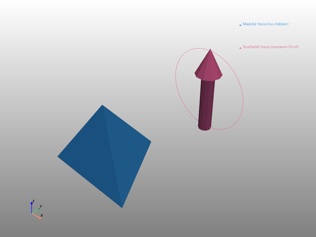
The following example shows how a generic trace is constructed with Mesh3d and Scatter3d and is displayed with three different backends:

import numpy as np
import pyvista as pv

import magpylib as magpy

# Mesh3d trace #########################

trace_mesh3d = {
    "backend": "generic",
    "constructor": "Mesh3d",
    "kwargs": {
        "x": (0.01, 0, -0.01, 0),
        "y": (-0.005, 0.012, -0.005, 0),
        "z": (-0.005, -0.005, -0.005, 0.01),
        "i": (0, 0, 0, 1),
        "j": (1, 1, 2, 2),
        "k": (2, 3, 3, 3),
        #'opacity': 0.5,
    },
}
coll = magpy.Collection(position=(0, -0.03, 0), style_label="'Mesh3d' trace")
coll.style.model3d.add_trace(trace_mesh3d)

# Scatter3d trace ######################

ts = np.linspace(0, 2 * np.pi, 30)
trace_scatter3d = {
    "backend": "generic",
    "constructor": "Scatter3d",
    "kwargs": {
        "x": np.cos(ts) / 100,
        "y": np.zeros(30),
        "z": np.sin(ts) / 100,
        "mode": "lines",
    },
}
dipole = magpy.misc.Dipole(
    moment=(0, 0, 1), style_label="'Scatter3d' trace", style_size=6
)
dipole.style.model3d.add_trace(trace_scatter3d)
# show the system using different backends
for backend in magpy.SUPPORTED_PLOTTING_BACKENDS:
    print(f"Plotting backend: {backend!r}")
    magpy.show(coll, dipole, backend=backend)

Plotting backend: 'matplotlib'

Plotting backend: 'plotly'

Plotting backend: 'pyvista'

/home/docs/checkouts/readthedocs.org/user_builds/magpylib/envs/stable/lib/python3.9/site-packages/pyvista/jupyter/notebook.py:34: UserWarning:

Failed to use notebook backend: 

No module named 'trame'

Falling back to a static output.

It is possible to have multiple user-defined traces that will be displayed at the same time. In addition, the following code shows how to quickly copy and manipulate trace dictionaries and Trace3d objects,

import copy

import numpy as np

import magpylib as magpy

ts = np.linspace(0, 2 * np.pi, 30)
trace_scatter3d = {
    "backend": "generic",
    "constructor": "Scatter3d",
    "kwargs": {
        "x": np.cos(ts) / 100,
        "y": np.zeros(30),
        "z": np.sin(ts) / 100,
        "mode": "lines",
    },
}
dipole = magpy.misc.Dipole(
    moment=(0, 0, 1),
    style_label="'Scatter3d' trace",
    style_size=0.01,
    style_sizemode="absolute",
)


# generate new trace from dictionary
trace2 = copy.deepcopy(trace_scatter3d)
trace2["kwargs"]["y"] = np.sin(ts) / 100
trace2["kwargs"]["z"] = np.zeros(30)

dipole.style.model3d.add_trace(trace2)

# generate new trace from Trace3d object
trace3 = copy.deepcopy(dipole.style.model3d.data[0])
trace3.kwargs["x"] = np.zeros(30)
trace3.kwargs["z"] = np.cos(ts) / 100

dipole.style.model3d.add_trace(trace3)

dipole.show(dipole, backend="matplotlib")

Matplotlib plotting functions often use positional arguments for \((x,y,z)\) input, that are handed over from args=(x,y,z) in trace. The following examples show how to construct traces with plot, plot_surface and plot_trisurf:

import matplotlib.pyplot as plt
import matplotlib.tri as mtri
import numpy as np

import magpylib as magpy

# plot trace ###########################

ts = np.linspace(-10, 10, 100)
xs = np.cos(ts) / 100
ys = np.sin(ts) / 100
zs = ts / 20 / 100

trace_plot = {
    "backend": "matplotlib",
    "constructor": "plot",
    "args": (xs, ys, zs),
    "kwargs": {"ls": "--", "lw": 2},
}
magnet = magpy.magnet.Cylinder(polarization=(0, 0, 1), dimension=(0.005, 0.01))
magnet.style.model3d.add_trace(trace_plot)

# plot_surface trace ###################

u, v = np.mgrid[0 : 2 * np.pi : 30j, 0 : np.pi : 20j]
xs = np.cos(u) * np.sin(v) / 100
ys = np.sin(u) * np.sin(v) / 100
zs = np.cos(v) / 100

trace_surf = {
    "backend": "matplotlib",
    "constructor": "plot_surface",
    "args": (xs, ys, zs),
    "kwargs": {"cmap": plt.cm.YlGnBu_r},
}
ball = magpy.Collection(position=(-0.03, 0, 0))
ball.style.model3d.add_trace(trace_surf)

# plot_trisurf trace ###################

u, v = np.mgrid[0 : 2 * np.pi : 50j, -0.5:0.5:10j]
u, v = u.flatten(), v.flatten()

xs = (1 + 0.5 * v * np.cos(u / 2.0)) * np.cos(u) / 100
ys = (1 + 0.5 * v * np.cos(u / 2.0)) * np.sin(u) / 100
zs = 0.5 * v * np.sin(u / 2.0) / 100

tri = mtri.Triangulation(u, v)

trace_trisurf = {
    "backend": "matplotlib",
    "constructor": "plot_trisurf",
    "args": (xs, ys, zs),
    "kwargs": {
        "triangles": tri.triangles,
        "cmap": plt.cm.coolwarm,
    },
}
mobius = magpy.misc.CustomSource(style_model3d_showdefault=False, position=(0.03, 0, 0))
mobius.style.model3d.add_trace(trace_trisurf)

magpy.show(magnet, ball, mobius, backend="matplotlib")

Pre-defined 3D models

Automatic trace generators are provided for several basic 3D models in magpylib.graphics.model3d. If no backend is specified, it defaults back to 'generic'. They can be used as follows,

import magpylib as magpy
from magpylib.graphics import model3d

# prism trace ###################################
trace_prism = model3d.make_Prism(
    base=6,
    diameter=0.02,
    height=0.01,
    position=(-0.03, 0, 0),
)
obj0 = magpy.Sensor(style_model3d_showdefault=False, style_label="Prism")
obj0.style.model3d.add_trace(trace_prism)

# pyramid trace #################################
trace_pyramid = model3d.make_Pyramid(
    base=30,
    diameter=0.02,
    height=0.01,
    position=(0.03, 0, 0),
)
obj1 = magpy.Sensor(style_model3d_showdefault=False, style_label="Pyramid")
obj1.style.model3d.add_trace(trace_pyramid)

# cuboid trace ##################################
trace_cuboid = model3d.make_Cuboid(
    dimension=(0.02, 0.02, 0.02),
    position=(0, 0.03, 0),
)
obj2 = magpy.Sensor(style_model3d_showdefault=False, style_label="Cuboid")
obj2.style.model3d.add_trace(trace_cuboid)

# cylinder segment trace ########################
trace_cylinder_segment = model3d.make_CylinderSegment(
    dimension=(0.01, 0.02, 0.01, 140, 220),
    position=(0.01, 0, -0.03),
)
obj3 = magpy.Sensor(style_model3d_showdefault=False, style_label="Cylinder Segment")
obj3.style.model3d.add_trace(trace_cylinder_segment)

# ellipsoid trace ###############################
trace_ellipsoid = model3d.make_Ellipsoid(
    dimension=(0.02, 0.02, 0.02),
    position=(0, 0, 0.03),
)
obj4 = magpy.Sensor(style_model3d_showdefault=False, style_label="Ellipsoid")
obj4.style.model3d.add_trace(trace_ellipsoid)

# arrow trace ###################################
trace_arrow = model3d.make_Arrow(
    base=30,
    diameter=0.006,
    height=0.02,
    position=(0, -0.03, 0),
)
obj5 = magpy.Sensor(style_model3d_showdefault=False, style_label="Arrow")
obj5.style.model3d.add_trace(trace_arrow)

magpy.show(obj0, obj1, obj2, obj3, obj4, obj5, backend="plotly")

Adding a CAD model

As shown in Special 3D models, it is possible to attach custom 3D model representations to any Magpylib object. In the example below we show how a standard CAD model can be transformed into a generic Magpylib graphic trace, and displayed by both matplotlib and plotly backends.

Note

The code below requires installation of the numpy-stl package.

import os
import tempfile

import numpy as np
import requests
from matplotlib.colors import to_hex
from stl import mesh  # requires installation of numpy-stl

import magpylib as magpy


def bin_color_to_hex(x):
    """transform binary rgb into hex color"""
    sb = f"{x:015b}"[::-1]
    r = int(sb[:5], base=2) / 31
    g = int(sb[5:10], base=2) / 31
    b = int(sb[10:15], base=2) / 31
    return to_hex((r, g, b))


def trace_from_stl(stl_file):
    """
    Generates a Magpylib 3D model trace dictionary from an *.stl file.
    backend: 'matplotlib' or 'plotly'
    """
    # load stl file
    stl_mesh = mesh.Mesh.from_file(stl_file)

    # extract vertices and triangulation
    p, q, r = stl_mesh.vectors.shape
    vertices, ixr = np.unique(
        stl_mesh.vectors.reshape(p * q, r), return_inverse=True, axis=0
    )
    i = np.take(ixr, [3 * k for k in range(p)])
    j = np.take(ixr, [3 * k + 1 for k in range(p)])
    k = np.take(ixr, [3 * k + 2 for k in range(p)])
    x, y, z = vertices.T

    # generate and return a generic trace which can be translated into any backend
    colors = stl_mesh.attr.flatten()
    facecolor = np.array([bin_color_to_hex(c) for c in colors]).T
    x, y, z = x / 1000, y / 1000, z / 1000  # mm->m
    trace = {
        "backend": "generic",
        "constructor": "mesh3d",
        "kwargs": dict(x=x, y=y, z=z, i=i, j=j, k=k, facecolor=facecolor),
    }
    return trace


# load stl file from online resource
url = "https://raw.githubusercontent.com/magpylib/magpylib-files/main/PG-SSO-3-2.stl"
file = url.split("/")[-1]
with tempfile.TemporaryDirectory() as temp:
    fn = os.path.join(temp, file)
    with open(fn, "wb") as f:
        response = requests.get(url)
        f.write(response.content)

    # create traces for both backends
    trace = trace_from_stl(fn)

# create sensor and add CAD model
sensor = magpy.Sensor(style_label="PG-SSO-3 package")
sensor.style.model3d.add_trace(trace)

# create magnet and sensor path
magnet = magpy.magnet.Cylinder(polarization=(0, 0, 1), dimension=(0.015, 0.02))
sensor.position = np.linspace((-0.015, 0, 0.008), (-0.015, 0, -0.004), 21)
sensor.rotate_from_angax(np.linspace(0, 180, 21), "z", anchor=0, start=0)

# display with matplotlib and plotly backends
args = (sensor, magnet)
kwargs = dict(style_path_frames=5)
magpy.show(args, **kwargs, backend="matplotlib")
magpy.show(args, **kwargs, backend="plotly")

---

[2]

possible but not implemented at the moment.

[7]

Matplotlib does not support color gradient. Instead magnetization is shown through object slicing and coloring.

[5] (1,2,3)

animation is only available through export as gif or mp4

[1]

when returning animation object and exporting it as jshtml.

[6]

2D plots are not supported for all jupyter_backends. As of pyvista>=0.38 these are deprecated and replaced by the trame backend.

[3]

only "scatter3d", and "mesh3d". Gets “translated” to every other backend.

[4]

custom user defined trace constructors allowed, which are specific to the backend.