
Get Started#
Installation and Dependencies#
Magpylib supports Python3.8+ and relies on common scientific computation libraries Numpy, Scipy, Matplotlib and Plotly. Optionally, Pyvista is recommended as graphical backend.
pip install magpylib
conda install -c conda-forge magpylib
Magpylib fundamentals#
Learn the Magpylib fundamentals in 5 minutes. This requires a basic understanding of the Python programming language, the Numpy array class and the Scipy Rotation class.
Step 1: Create sources and observers as Python objects#
import magpylib as magpy

# Create a Cuboid magnet with magnetic polarization
# of 1 T pointing in x-direction and sides of
# 1,2 and 3 cm respectively (notice the use of SI units).

cube = magpy.magnet.Cuboid(polarization=(1,0,0), dimension=(0.01,0.02,0.03))

# Create a Sensor for measuring the field

sensor = magpy.Sensor()
Step2: Manipulate object position and orientation#
# By default, the position of a Magpylib object is
# (0,0,0) and its orientation is the unit rotation,
# given by a scipy rotation object.

print(cube.position)                   # -> [0. 0. 0.]
print(cube.orientation.as_rotvec())    # -> [0. 0. 0.]

# Manipulate object position and orientation through
# the respective attributes (move 10 mm and rotate 45 deg):

from scipy.spatial.transform import Rotation as R
cube.position = (0.01,0,0)
cube.orientation = R.from_rotvec((0,0,45), degrees=True)

print(cube.position)                            # -> [0.01 0.   0.  ]
print(cube.orientation.as_rotvec(degrees=True)) # -> [0. 0. 45.]

# Apply relative motion with the powerful `move`
# and `rotate` methods.
sensor.move((-0.01,0,0))
sensor.rotate_from_angax(angle=-45, axis='z')

print(sensor.position)                            # -> [-0.01  0.    0.  ]
print(sensor.orientation.as_rotvec(degrees=True)) # -> [ 0.  0. -45.]
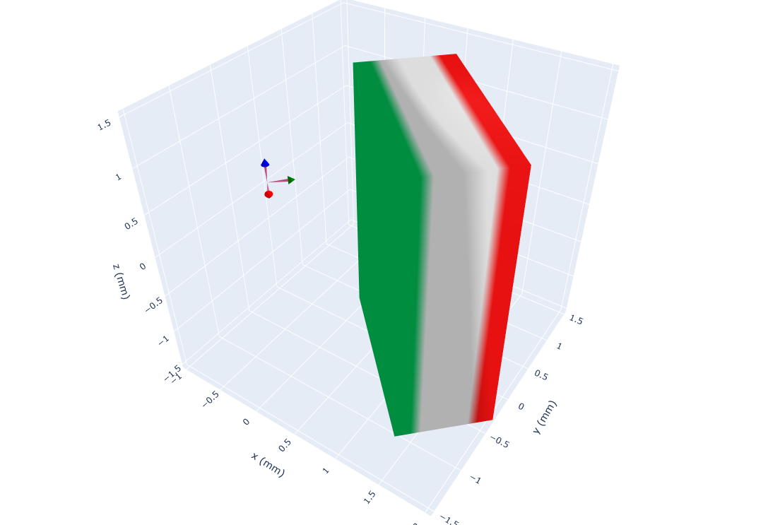
Step 3: View your system#
# Use the `show` function to view your system
# through Matplotlib, Plotly or Pyvista backends.

magpy.show(cube, sensor, backend='plotly')
Step 4: Computing the field#
# Compute the B-field in units of T for some points.

points = [(0,0,-.01), (0,0,0), (0,0,.01)] # in SI Units (m)
B = magpy.getB(cube, points)

print(B.round(2)) # -> [[ 0.26  0.07  0.08]
                     # [ 0.28  0.05  0.  ]
                     # [ 0.26  0.07 -0.08]] # in SI Units (T)

# Compute the H-field in units of A/m at the sensor.

H = magpy.getH(cube, sensor)

print(H.round()) # -> [51017. 24210.     0.] # in SI Units (A/m)
Warning
Magpylib makes use of vectorized computation (massive speedup). This requires that you hand over all field computation instances (multiple objects with multiple positions (=paths)) at the same time to getB, getH, getJ and getM. Avoid Python loops at all costs !!!
Other important features#
Paths
Magpylib position and orientation attributes can store multiple values that are referred to as paths. The field will automatically be computed for all path positions. Use this to model objects that move to multiple locations.
import numpy as np
import magpylib as magpy

# Create magnet
sphere = magpy.magnet.Sphere(
    diameter=.01,
    polarization=(0,0,1)
)

# Assign a path
sphere.position = np.linspace((-.02,0,0), (.02,0,0), 7)

# The field is automatically computed for every path position
B = sphere.getB((0,0,.01))
print(B.round(3))  # ->[[ 0.004  0.    -0.001]
                      # [ 0.013  0.     0.001]
                      # [ 0.033  0.     0.026]
                      # [ 0.     0.     0.083]
                      # [-0.033  0.     0.026]
                      # [-0.013  0.     0.001]
                      # [-0.004  0.    -0.001]]
Collections
Magpylib objects can be grouped into Collections. An operation applied to a Collection is applied to every object in it.
import magpylib as magpy

# Create objects
obj1 = magpy.Sensor()
obj2 = magpy.magnet.Cuboid(
    polarization=(0,0,1),
    dimension=(.01,.02,.03))

# Group objects
coll = magpy.Collection(obj1, obj2)

# Manipulate Collection
coll.move((.001,.002,.003))

print(obj1.position) # -> [0.001 0.002 0.003]
print(obj2.position) # -> [0.001 0.002 0.003]
Complex Magnet Shapes
There most convenient way to create a magnet with complex shape is by using the convex hull of a point cloud (= simplest form that includes all given points) and transform it into a triangular surface mesh.
import numpy as np

import magpylib as magpy

# Create a Pyramid magnet
points = (
    np.array(
        [
            (-1, -1, 0),
            (-1, 1, 0),
            (1, -1, 0),
            (1, 1, 0),
            (0, 0, 2),
        ]
    )
)
pyramid = magpy.magnet.TriangularMesh.from_ConvexHull(
    magnetization=(0, 0, 1e6),
    points=points,
)

# Display the magnet graphically
pyramid.show()
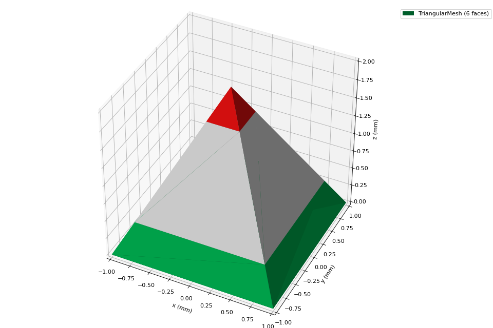
However, there are several other possibilities to create complex magnet shapes. Some can be found in the gallery.
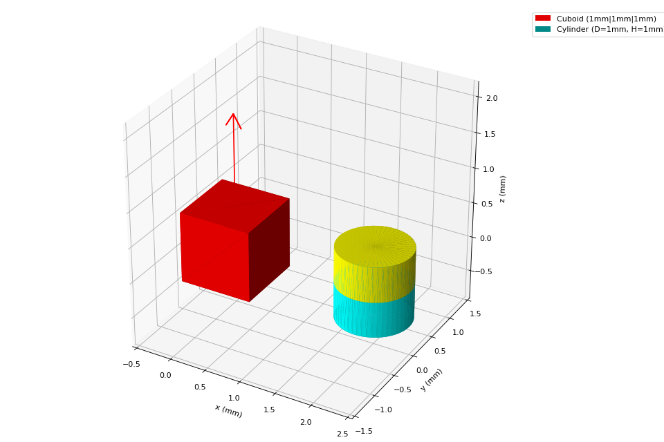
Graphic Styles
Magpylib offers many ways to customize the graphic output.
import magpylib as magpy

# create Cuboid magnet with custom style
cube = magpy.magnet.Cuboid(
    polarization=(0,0,1),
    dimension=(.01,.01,.01),
    style_color='r',
    style_magnetization_mode='arrow'
)

# create Cylinder magnet with custom style
cyl = magpy.magnet.Cylinder(
    polarization=(0,0,1),
    dimension=(.01,.01),
    position=(.02,0,0),
    style_magnetization_color_mode='bicolor',
    style_magnetization_color_north='m',
    style_magnetization_color_south='c',
)
magpy.show(cube, cyl)
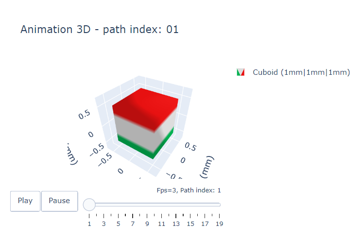
Animation
Object paths can be animated
import numpy as np
import magpylib as magpy


# Create magnet with path
cube = magpy.magnet.Cuboid(
    magnetization=(0,0,1),
    dimension=(1,1,1),
)
cube.rotate_from_angax(
    angle=np.linspace(10,360,18),
    axis='x'
)

# Generate an animation with `show`
cube.show(animation=True, backend="plotly")
Functional interface
Magpylib’s object oriented interface is convenient to work with but is also slowed down by object initialization and handling. The functional interface bypasses this load and enables field computation for a set of input parameters.
import magpylib as magpy

# Compute the magnetic field via the functional interface.
B = magpy.getB(
    sources="Cuboid",
    observers=[(-1, 0, 1), (0, 0, 1), (1, 0, 1)],
    dimension=(1, 1, 1),
    polarization=(0, 0, 1),
)

print(B.round(3))  # -> [[-0.043  0.     0.014]
                       # [ 0.     0.     0.135]
                       # [ 0.043  0.     0.014]]