Magpylib API

Magpylib API#

Types#

Magpylib requires no special input format. All scalar types (int, float, …) and vector types (list, tuple, np.ndarray, … ) are accepted. Magpylib returns everything as np.ndarray.

Units#

The important vacuum permeability \(\mu_0\) is provided at the package top-level mu_0. It’s value is not \(4 \pi 10^{-7}\) since the redefinition of the SI base units, but a value close to it.

For historical reasons Magpylib used non-SI units until Version 4. Starting with version 5 all inputs and outputs are SI-based.

PHYSICAL QUANTITY	MAGPYLIB PARAMETER	UNITS from v5	UNITS until v4
Magnetic Polarization \(\vec{J}\)	`polarization`, `getJ()`	T	-
Magnetization \(\vec{M}\)	`magnetization`, `getM()`	A/m	mT
Electric Current \(i_0\)	`current`	A	A
Magnetic Dipole Moment \(\vec{m}\)	`moment`	A·m²	mT·mm³
B-field \(\vec{B}\)	`getB()`	T	mT
H-field \(\vec{H}\)	`getH()`	A/m	kA/m
Length-inputs	`position`, `dimension`, `vertices`, …	m	mm
Angle-inputs	`angle`, `dimension`, …	°	°

Warning

Up to version 4, Magpylib was unfortunately contributing to the naming confusion in magnetism that is explained well here. The input magnetization in Magpylib < v5 was referring to the magnetic polarization (and not the magnetization), the difference being only in the physical unit. From version 5 onwards this is fixed.

Hint

All input and output units in Magpylib (version 5 and higher) are SI-based, see table above. However, for advanced use one should be aware that the analytical solutions are scale invariant - “a magnet with 1 mm sides creates the same field at 1 mm distance as a magnet with 1 m sides at 1 m distance”. The choice of length input unit is therefore not relevant, but it is critical to keep the same length unit for all inputs in one computation.

In addition, getB returns the same unit as given by the polarization input. With polarization input in mT, getB will return mT as well. At the same time when the magnetization input is kA/m, then getH returns kA/m as well. The B/H-field outputs are related to a M/J-inputs via a factor of \(µ_0\).

Note

The connection between the magnetic polarization J, the magnetization M and the material parameters of a real permanent magnet are shown in Modelling a real magnet.

The Magpylib Classes#

In Magpylib’s object oriented interface magnetic field sources (generate the field) and observers (read the field) are created as Python objects with various defining attributes and methods.

Base properties#

The following basic properties are shared by all Magpylib classes:

The position and orientation attributes describe the object placement in the global coordinate system.
The move() and rotate() methods enable relative object positioning.
The reset_path() method sets position and orientation to default values.
The barycenter property returns the object barycenter (often the same as position).

See Position, Orientation, and Paths for more information on these features.

The style attribute includes all settings for graphical object representation.
The show() method gives quick access to the graphical representation.

See Graphics for more information on graphic output, default styles and customization possibilities.

The getB(), getH(), getJ() and getM() methods give quick access to field computation.

See Field Computation for more information.

The parent attribute references a Collection that the object is part of.
The copy() method creates a clone of any object where selected properties, given by kwargs, are modified.
The describe() method provides a brief description of the object and returns the unique object id.

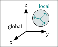
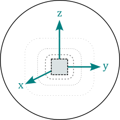
Local and global coordinates#

Magpylib objects span a local reference frame, and all object properties are defined within this frame, for example the vertices of a Tetrahedron magnet. The position and orientation attributes describe how the local frame lies within the global coordinates. The two frames coincide by default, when position=(0,0,0) and orientation=None (=unit rotation). The position and orientation attributes are described in detail in Position, Orientation, and Paths.

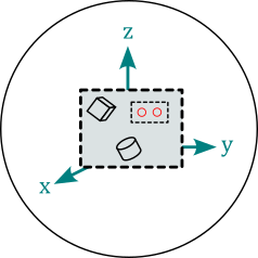
Magnet classes#

All magnets are sources. They have the polarization attribute which is of the format \(\vec{J}=(J_x, J_y, J_z)\) and denotes a homogeneous magnetic polarization vector in the local object coordinates in units of T. Alternatively, the magnetization vector can be set via the magnetization attribute of the format \(\vec{M}=(M_x, M_y, M_z)\). These two parameters are codependent and Magpylib ensures that they stay in sync via the relation \(\vec{J}=\mu_0\cdot\vec{M}\). Information on how this is related to material properties from data sheets is found in Modelling a real magnet.

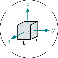
Cuboid#

magpylib.magnet.Cuboid(position, orientation, dimension, polarization, magnetization, style)

Cuboid objects represent magnets with cuboid shape. The dimension attribute has the format \((a,b,c)\) and denotes the sides of the cuboid units of meter. The center of the cuboid lies in the origin of the local coordinates, and the sides are parallel to the coordinate axes.

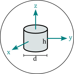
Cylinder#

magpylib.magnet.Cylinder(position, orientation, dimension, polarization, magnetization, style)

Cylinder objects represent magnets with cylindrical shape. The dimension attribute has the format \((d,h)\) and denotes diameter and height of the cylinder in units of meter. The center of the cylinder lies in the origin of the local coordinates, and the cylinder axis coincides with the z-axis.

CylinderSegment#

magpylib.magnet.CylinderSegment(position, orientation, dimension, polarization, magnetization, style)

CylinderSegment objects represent magnets with the shape of a cylindrical ring section. The dimension attribute has the format \((r_1,r_2,h,\varphi_1,\varphi_2)\) and denotes inner radius, outer radius and height in units of meter, and the two section angles \(\varphi_1<\varphi_2\) in °. The center of the full cylinder lies in the origin of the local coordinates, and the cylinder axis coincides with the z-axis.

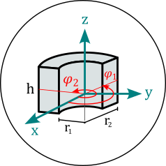
Info: When the cylinder section angles span 360°, then the much faster Cylinder methods are used for the field computation.

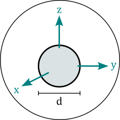
Sphere#

magpylib.magnet.Sphere(position, orientation, diameter, polarization, magnetization, style)

Sphere objects represent magnets of spherical shape. The diameter attribute is the sphere diameter \(d\) in units of meter. The center of the sphere lies in the origin of the local coordinates.

Tetrahedron#

magpylib.magnet.Tetrahedron(position, orientation, vertices, polarization, magnetization, style)

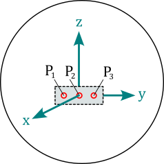
Tetrahedron objects represent magnets of tetrahedral shape. The vertices attribute stores the four corner points \((\vec{P}_1, \vec{P}_2, \vec{P}_3, \vec{P}_4)\) in the local object coordinates in units of m.

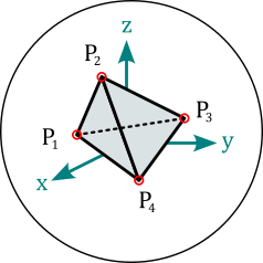
Info: The Tetrahedron field is computed from four Triangle fields.

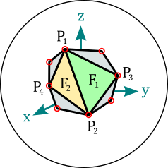
TriangularMesh#

magpylib.magnet.TriangularMesh(position, orientation, vertices, faces, polarization, magnetization, check_open, check_disconnected, check_selfintersecting, reorient_faces, style)

TriangularMesh objects represent magnets with surface given by a triangular mesh. The mesh is defined by the vertices attribute, an array of all unique corner points \((\vec{P}_1, \vec{P}_2, ...)\) in units of meter, and the faces attribute, which is an array of index-triplets that define individual faces \((\vec{F}_1, \vec{F}_2, ...)\). The property mesh returns an array of all faces as point-triples \([(\vec{P}_1^1, \vec{P}_2^1, \vec{P}_3^1), (\vec{P}_1^2, \vec{P}_2^2, \vec{P}_3^2), ...]\).

At initialization the mesh integrity is automatically checked, and all faces are reoriented to point outwards. These actions are controlled via the kwargs

check_open
check_disconnected
check_selfintersecting
reorient_faces

which are all by default set to "warn". Options are "skip" (don’t perform check), "ignore" (ignore if check fails), "warn" (warn if check fails), "raise" (raise error if check fails).

Results of the checks are stored in the following object attributes

status_open can be True, False or None (unchecked)
status_open_data contains an array of open edges
status_disconnected can be True, False or None (unchecked)
status_disconnected_data contains an array of mesh parts
status_selfintersecting can be True, None or None (unchecked)
status_selfintersecting_data contains an array of self-intersecting faces
status_reoriented can be True or False

The checks can also be performed after initialization using the methods

check_open()
check_disconnected()
check_selfintersecting()
reorient_faces()

The following class methods enable easy mesh creating and mesh loading.

TriangularMesh.from_mesh() generates a TriangularMesh objects from the input mesh, which is an array in the mesh format \([(\vec{P}_1^1, \vec{P}_2^1, \vec{P}_3^1), (\vec{P}_1^2, \vec{P}_2^2, \vec{P}_3^2), ...]\).
TriangularMesh.from_ConvexHull() generates a TriangularMesh object from the input points, which is an array of positions \((\vec{P}_1, \vec{P}_2, \vec{P}_3, ...)\) from which the convex Hull is computed via the Scipy ConvexHull implementation.
TriangularMesh.from_triangles() generates a TriangularMesh object from the input triangles, which is a list or a Collection of Triangle objects.
TriangularMesh.from_pyvista() generates a TriangularMesh object from the input polydata, which is a Pyvista PolyData object.

The method to_TriangleCollection() transforms a TriangularMesh object into a Collection of Triangle objects.

Info: While the checks may be disabled, the field computation guarantees correct results only if the mesh is closed, connected, not self-intersecting and all faces are oriented outwards. Examples of working with the TriangularMesh class are found in Triangular Meshes and in Pyvista Bodies.

Current classes#

All currents are sources. Current objects have the current attribute which is a scalar that denotes the electrical current in units of ampere.

Circle#

magpylib.current.Circle(position, orientation, diameter, current, style)

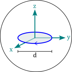
Circle objects represent circular line current loops. The diameter attribute is the loop diameter \(d\) in units of meter. The loop lies in the xy-plane with it’s center in the origin of the local coordinates.

Polyline#

magpylib.current.Polyline(position, orientation, vertices, current, style)

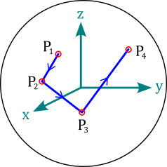
Polyline objects represent line current segments where the electric current flows in straight lines from vertex to vertex. The vertices attribute is a vector of all vertices \((\vec{P}_1, \vec{P}_2, ...)\) given in the local coordinates in units of meter.

Miscellaneous classes#

There are classes listed hereon that function as sources, but they do not represent physical magnets or current distributions.

Dipole#

magpylib.misc.Dipole(position, orientation, moment, style)

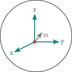
Dipole objects represent magnetic dipole moments with the moment attribute that describes the magnetic dipole moment \(\vec{m}=(m_x,m_y,m_z)\) in SI-units of Am², which lies in the origin of the local coordinates.

Info: The total dipole moment of a homogeneous magnet with body volume \(V\) is given by \(\vec{m}=\vec{J}\cdot V\).

Triangle#

magpylib.misc.Triangle(position, orientation, vertices, polarization, magnetization, style)

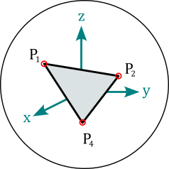
Triangle objects represent triangular surfaces with homogeneous charge density given by the projection of the polarization or magnetization vector onto the surface normal. The attributes polarization and magnetization are treated similar as by the Magnet classes. The vertices attribute is a set of the three triangle corners \((\vec{P}_1, \vec{P}_2, \vec{P}_3)\) in units of meter in the local coordinates.

Info: When multiple Triangles with similar magnetization/polarization vectors form a closed surface, and all their orientations (right-hand-rule) point outwards, their total H-field is equivalent to the field of a homogeneous magnet of the same shape. In this case, the B-field is only correct on the outside of the body. On the inside the polarization must be added to the field. This is demonstrated in the tutorial Triangular Meshes.

CustomSource#

magpylib.misc.CustomSource(field_func, position, orientation, style)

The CustomSource class is used to create user defined sources provided with with custom field computation functions. The argument field_func takes a function that is then automatically called for the field computation. This custom field function is treated like a core function. It must have the positional arguments field with values "B" or "H", and observers (must accept array with shape (n,3)) and return the B-field and the H-field with a similar shape.

Info: A tutorial CustomSource is found in the gallery.

Sensor#

magpylib.Sensor(position, orientation, pixel, handedness, style)

Sensor objects represent observers of the magnetic field and can be used as Magpylib observers input for magnetic field computation. The pixel attribute is an array of positions \((\vec{P}_1, \vec{P}_2, ...)\) provided in units of meter in the local sensor coordinates. A sensor returns the magnetic field at these pixel positions. By default pixel=(0,0,0) and the sensor simply returns the field at it’s position. The handedness attribute can be "left" or "right" (default) to set a left- or right-handed sensor coordinate system for the field computation.

Info: Sensors can have their own position and orientation and enable easy relative positioning between sources and observers. The field is always computed in the reference frame of the sensor, which might itself be moving in the global coordinate system. Magpylib sensors can be understood as perfect magnetic field sensors with infinitesimally sensitive elements. An example how to use sensors is given in Using Sensors.

Collection#

magpylib.Collection(*children, position, orientation, override_parent, style)

A Collection is a group of Magpylib objects that is used for common manipulation. All these objects are stored by reference in the children attribute. The collection becomes the parent of the object. An object can only have one parent. There are several options for accessing only specific children via the following properties

sources: return only sources
observers: return only observers
collections: return only collections
sources_all: return all sources, including the ones from sub-collections
observers_all: return all observers, including the ones from sub-collections
collections_all: return all collections, including the ones from sub-collections

Additional methods for adding and removing children:

add(): Add an object to the collection
remove(): Remove an object from the collection

Info: A collection object has its own position and orientation attributes and spans a local reference frame for all its children. An operation applied to a collection moves the frame, and is individually applied to all children such that their relative position in the local reference frame is maintained. This means that the collection functions as a container for manipulation, but child position and orientation are always updated in the global coordinate system. After being added to a collection, it is still possible to manipulate the individual children, which will also move them to a new relative position in the collection frame.

Collections have format as an additional argument for describe() method. Default value is format="type+id+label". Any combination of "type", "id", and "label" is allowed.

A tutorial Working with Collections is provided in the example gallery.

Position, Orientation, and Paths#

The explicit magnetic field expressions found in the literature, implemented in the Magpylib core, are given in convenient source-coordinates. It is a common problem to transform the field into an application relevant observer coordinate system. While not technically difficult, such transformations are prone to error.

Here Magpylib helps out. All Magpylib sources and observers lie in a global Cartesian coordinate system. Object position and orientation are defined by the attributes position and orientation, 😏. Objects can easily be moved around using the move() and rotate() methods. Eventually, the field is computed in the reference frame of the observers (e.g. Sensor objects). Positions are given in units of meter, and the default unit for orientation is °.

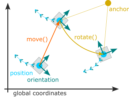
Position and orientation of all Magpylib objects are defined by the two attributes

position - a point \((x,y,z)\) in the global coordinates, or a set of such points \((\vec{P}_1, \vec{P}_2, ...)\). By default objects are created with position=(0,0,0).

orientation - a Scipy Rotation object which describes the object rotation relative to its default orientation (defined in The Magpylib Classes). By default, objects are created with unit rotation orientation=None.

The position and orientation attributes can be either scalar, i.e. a single position or a single rotation, or vector, when they are arrays of such scalars. The two attributes together define the path of an object - Magpylib makes sure that they are always of the same length. When the field is computed, it is automatically computed for the whole path.

Tip

To enable vectorized field computation, paths should always be used when modeling multiple object positions. Avoid using Python loops at all costs for that purpose! If your path is difficult to realize, consider using the functional interface instead.

Magpylib offers two powerful methods for object manipulation:

move(displacement, start="auto") - move object by displacement input. displacement is a position vector (scalar input) or a set of position vectors (vector input).

rotate(rotation, anchor=None, start="auto") - rotates the object by the rotation input about an anchor point defined by the anchor input. rotation is a Scipy Rotation object, and anchor is a position vector. Both can be scalar or vector inputs. With anchor=None the object is rotated about its position.

Scalar input is applied to the whole object path, starting with path index start. With the default start="auto" the index is set to start=0 and the functionality is moving objects around (incl. their whole paths).
Vector input of length \(n\) applies the \(n\) individual operations to \(n\) object path entries, starting with path index start. Padding applies when the input exceeds the existing path length. With the default start="auto" the index is set to start=len(object path) and the functionality is appending the input.

The practical application of this formalism is best demonstrated by the following program

import magpylib as magpy
# Note that all units are in SI

sensor = magpy.Sensor()
print(sensor.position)                                    # default value
#   --> [0. 0. 0.]

sensor.move((1,1,1))                                      # scalar input is by default applied
print(sensor.position)                                    # to the whole path
#   --> [1. 1. 1.]

sensor.move([(1,1,1), (2,2,2)])                           # vector input is by default appended
print(sensor.position)                                    # to the existing path
#   --> [[1. 1. 1.]  [2. 2. 2.]  [3. 3. 3.]]

sensor.move((1,1,1), start=1)                             # scalar input and start=1 is applied
print(sensor.position)                                    # to whole path starting at index 1
#   --> [[1. 1. 1.]  [3. 3. 3.]  [4. 4. 4.]]

sensor.move([(0,0,10), (0,0,20)], start=1)                # vector input and start=1 merges
print(sensor.position)                                    # the input with the existing path
#   --> [[ 1.  1.  1.]  [ 3.  3. 13.]  [ 4.  4. 24.]]     # starting at index 1.

Several extensions of the rotate method give a lot of flexibility with object rotation. They all feature the arguments anchor and start which work as described above.

When objects with different path lengths are combined, e.g. when computing the field, the shorter paths are treated as static beyond their end to make the computation sensible. Internally, Magpylib follows a philosophy of edge-padding and end-slicing when adjusting paths.

Edge-padding: whenever path entries beyond the existing path length are needed the edge-entries of the existing path are returned. This means that the object is considered to be “static” beyond its existing path.

End-slicing: whenever a path is automatically reduced in length, Magpylib will slice such that the ending of the path is kept.

The tutorial Working with Paths shows intuitive good practice examples of the important functionality described in this section.

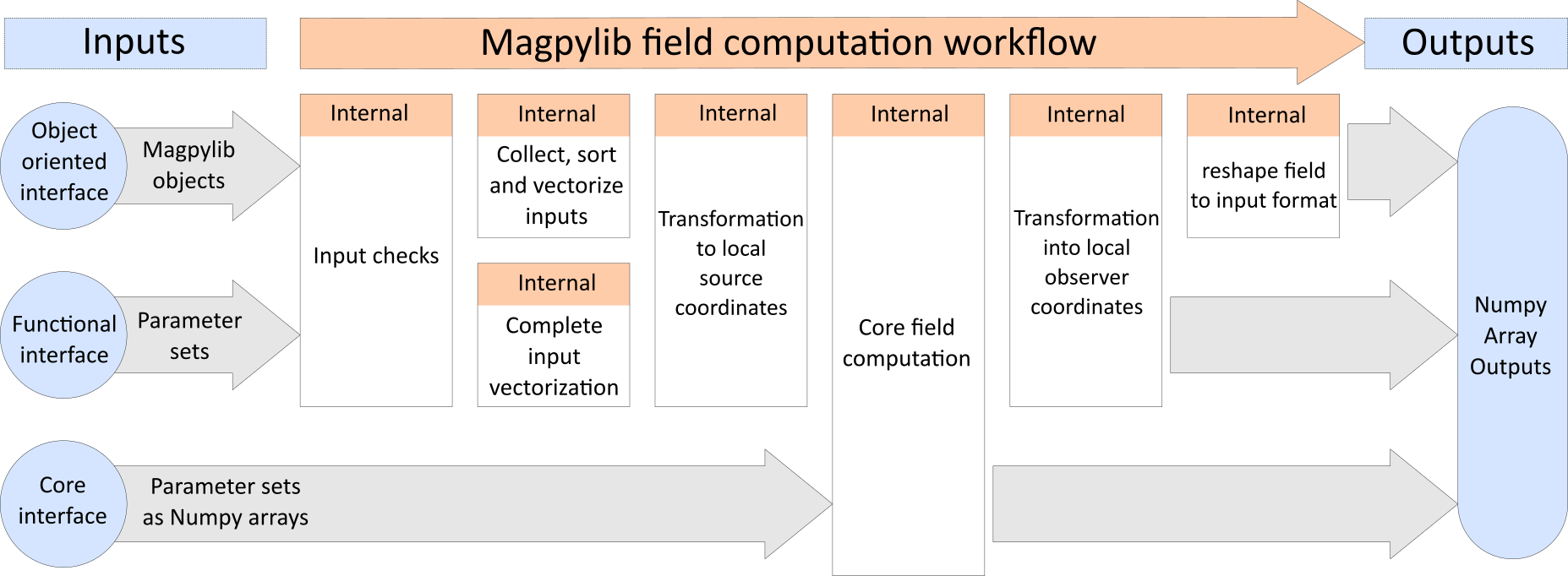
Field Computation#

Magnetic field computation in Magpylib is done via four top-level functions getB, getH, getJ and, getM,

magpylib.getB(sources, observers, squeeze=True, pixel_agg=None, output="ndarray")
magpylib.getH(sources, observers, squeeze=True, pixel_agg=None, output="ndarray")
magpylib.getJ(sources, observers, squeeze=True, pixel_agg=None, output="ndarray")
magpylib.getM(sources, observers, squeeze=True, pixel_agg=None, output="ndarray")

that compute the respective field generated by sources as seen by the observers in their local coordinates. sources can be any Magpylib source object (e.g. magnets) or a flat list thereof. observers can be an array of position vectors with shape (n1,n2,n3,...,3), any Magpylib observer object (e.g. sensors), or a flat list thereof. For quick-access, the functions getBHJM are also methods of all Magpylib objects, such that the sources or observers input is the object itself.

The following code shows a minimal example for Magpylib field computation.

import magpylib as magpy
# All inputs and outputs in SI units

# define source and observer objects
loop = magpy.current.Circle(current=1, diameter=.001)
sens = magpy.Sensor()

# compute field
B = magpy.getB(loop, sens)

print(B)
#  --> [0.         0.         0.00125664]

By default, getB returns the B-field in units of T, getH the H-field in units of A/m, getJ the magnetic polarization in T and, getM the magnetization in A/m, assuming that all inputs are given in SI units as described in the docstrings.

Note

In reality, getB returns the same unit as given by the polarization input. For example, with polarization input in mT, getB will return mT as well. At the same time when the magnetization input is kA/m, then getH returns kA/m as well. The B/H-field outputs are related to a M/J-inputs via a factor of \(µ_0\).

The output of a field computation magpy.getB(sources, observers) is by default a Numpy array of shape (l, m, k, n1, n2, n3, ..., 3) where l is the number of input sources, m the (maximal) object path length, k the number of observers, n1,n2,n3,... the sensor pixel shape or the shape of the observer position array input and 3 the three magnetic field components \((B_x, B_y, B_z)\).

squeeze: If True (default) all axes of length 1 in the output (e.g. only a single source) are squeezed.
pixel_agg: Select a compatible numpy aggregator function (e.g. "min", "mean") that is applied to the output. For example, with pixel_agg="mean" the mean field of all observer points is returned. With this option it is possible to supply getBHJM with multiple observers that have different pixel shapes.
output: Change the output format. Options are "ndarray" (default, returns a Numpy ndarray) and "dataframe" (returns a 2D-table Pandas DataFrame).

Note

Magpylib collects all inputs (object parameters), and vectorizes them for the computation which reduces the computation time dramatically for large inputs.

Try to make all field computations with as few calls to getBHJM as possible. Avoid Python loops at all costs!

The tutorial Computing the Field shows good practices with Magpylib field computation.

Functional interface#

Users can bypass the object oriented functionality of Magpylib and instead compute the field for n given parameter sets. This is done by providing the following inputs to the top level functions getB, getH, getJ and, getM.

sources: a string denoting the source type. Allowed values are the Magpylib source class names, see The Magpylib Classes.
observers: array-like of shape (3,) or (n,3) giving the observer positions.
kwargs: a dictionary with inputs of shape (x,) or (n,x). Must include all mandatory class-specific inputs. By default, position=(0,0,0) and orientation=None(=unit rotation).

All “scalar” inputs of shape (x,) are automatically tiled up to shape (n,x) to create a set of n computation instances. The field is returned in the shape (n,3). The following code demonstrates the functional interface.

import numpy as np
import magpylib as magpy
# All inputs and outputs in SI units

# compute the cuboid field for 3 input instances
N = 3 # number of instances
B = magpy.getB(
    sources='Cuboid',
    observers=np.linspace((0,0,1), (0,0,3), N),
    dimension=np.linspace((1,1,1), (3,3,3),3, N),
    polarization=(0,0,1),
)

# This example demonstrates the scale invariance
print(B)
#  --> [[0.         0.         0.13478239]
#       [0.         0.         0.13478239]
#       [0.         0.         0.13478239]]

Note

The functional interface is potentially faster than the object oriented one if users know how to generate the input arrays efficiently with numpy (e.g. np.arange, np.linspace, np.tile, np.repeat, …).

Core interface#

At the heart of Magpylib lies a set of core functions that are our implementations of explicit field expressions found in the literature, see Physics. Direct access to these functions is given through the magpylib.core subpackage which includes,

magnet_cuboid_Bfield( observers, dimensions, polarizations)

magnet_cylinder_axial_Bfield( z0, r, z)

magnet_cylinder_diametral_Hfield( z0, r, z, phi)

magnet_cylinder_segment_Hfield( observers, dimensions, magnetizations)

magnet_sphere_Bfield(observers, diameters, polarizations)

current_circle_Hfield(r0, r, z, i0)

current_polyline_Hfield(observers, segments_start, segments_end, currents)

dipole_Hfield(observers, moments)

triangle_Bfield(observers, vertices, polarizations)

All inputs must be Numpy ndarrays of shape (n,x). Details can be found in the respective function docstrings. The following example demonstrates the core interface.

import numpy as np
import magpylib as magpy
# All inputs and outputs in SI units

# prepare input
z0 = np.array([1,1])
r  = np.array([1,1])
z  = np.array([2,2])

# compute field with core functions
B = magpy.core.magnet_cylinder_axial_Bfield(z0=z0, r=r, z=z).T

print(B)
#  --> [[0.05561469 0.         0.06690167]
#       [0.05561469 0.         0.06690167]]

Field computation workflow#

The Magpylib field computation internal workflow and different approaches of the three interfaces is outlined in the following sketch.

Magpylib API

Contents

Magpylib API#

Types#

Units#

The Magpylib Classes#

Base properties#

Local and global coordinates#

Magnet classes#

Cuboid#

Cylinder#

CylinderSegment#

Sphere#

Tetrahedron#

TriangularMesh#

Current classes#

Circle#

Polyline#

Miscellaneous classes#

Dipole#

Triangle#

CustomSource#

Sensor#

Collection#

Position, Orientation, and Paths#

Field Computation#

Functional interface#

Core interface#

Field computation workflow#