What is magpylib ?
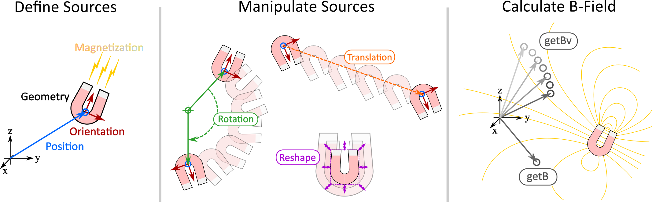
- Free Python package for calculating magnetic fields of magnets, currents and moments (sources).
- Provides convenient methods to create, geometrically manipulate, group and visualize assemblies of sources.
- The magnetic fields are determined from underlying analytical solutions which results in fast computation times and requires little computation power.
- For high performance computation (e.g. for multivariate parameter space analysis) all functions are also available in vectorized form.
Quickstart
Install magpylib with pip: >> pip install magpylib.
Example:
Run this simple code to calculate the magnetic field of a cylindrical magnet.
from magpylib.source.magnet import Cylinder
s = Cylinder( mag = [0,0,350], dim = [4,5])
print(s.getB([4,4,4]))

# Output: [ 5.08641867  5.08641867 -0.60532983]
In this example the cylinder axis is parallel to the z-axis. The diameter and height of the magnet are 4 millimeter and 5 millimeter respectively and the magnet position (=geometric center) is in the origin. The magnetization / remanence field is homogeneous and points in z-direction with an amplitude of 350 millitesla. Finally, the magnetic field B is calculated in units of millitesla at the positition [4,4,4] millimeter.
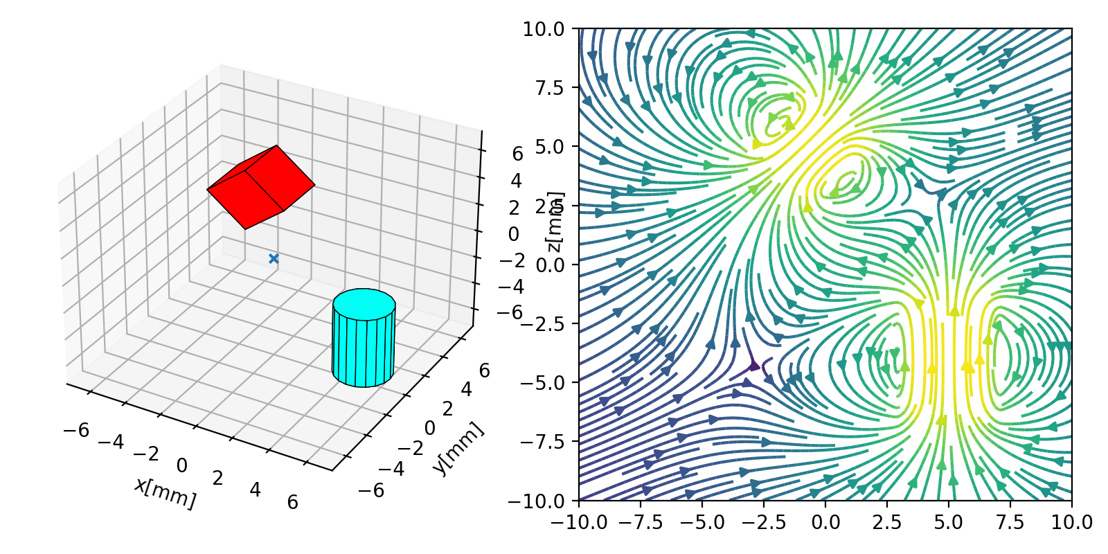
Example:
The following code calculates the combined field of two magnets. They are geometrically manipulated, the system geometry is displayed together with the field in the xz-plane.
# imports
import numpy as np
import matplotlib.pyplot as plt
import magpylib as magpy

# create figure
fig = plt.figure(figsize=(8,4))
ax1 = fig.add_subplot(121, projection='3d')  # this is a 3D-plotting-axis
ax2 = fig.add_subplot(122)                   # this is a 2D-plotting-axis

# create magnets
s1 = magpy.source.magnet.Box(mag=[0,0,600],dim=[3,3,3],pos=[-4,0,3])
s2 = magpy.source.magnet.Cylinder(mag=[0,0,500], dim=[3,5])

# manipulate magnets
s1.rotate(45,[0,1,0],anchor=[0,0,0])
s2.move([5,0,-4])

# create collection
c = magpy.Collection(s1,s2)

# display system geometry on ax1
magpy.displaySystem(c,subplotAx=ax1,suppress=True)

# calculate B-field on a grid
xs = np.linspace(-10,10,29)
zs = np.linspace(-10,10,29)
Bs = np.array([[c.getB([x,0,z]) for x in xs] for z in zs])

# display field in xz-plane using matplotlib
X,Z = np.meshgrid(xs,zs)
U,V = Bs[:,:,0], Bs[:,:,2]
ax2.streamplot(X, Z, U, V, color=np.log(U**2+V**2),density=2)

plt.show()
(Source code, png, hires.png, pdf)

More examples can be found in the Examples Section.
Technical details can be found in the Documentation v2.0.1b .
Content:
Library Docstrings: