Documentation v2.0.1b¶

The idea behind magpylib is to provide a simple and easy-to-use interface for computing the magnetic field of magnets, currents and moments. The computations are based on (semi-)analytical solutions found in the literature, discussed in the [WIP] Physics & Computation section.

Contents¶

Package Structure
Units and IO types
The Source Class
Calculating the Magnetic Field
- Using magpylib.vector
Collections
The Sensor Class
Display System Graphically
Math Package

Package Structure¶

The top level of magpylib contains the sub-packages and source, vector and math, the classes magpylib.Collection and magpylib.Sensor as well as the function magpylib.displaySystem().

The source module includes a set of classes that represent physical sources of the magnetic field (e.g. permanent magnets).
The vector module includes functions for performance computation.
The math module contains practical functions for working with angle-axis rotations and transformation to and from Euler angle representation.
The Collection class is used to group sources and for common manipulation.
The Sensor class represents a 3D magnetic sensor.
The displaySystem function is used to create a graphical output of the system geometry.

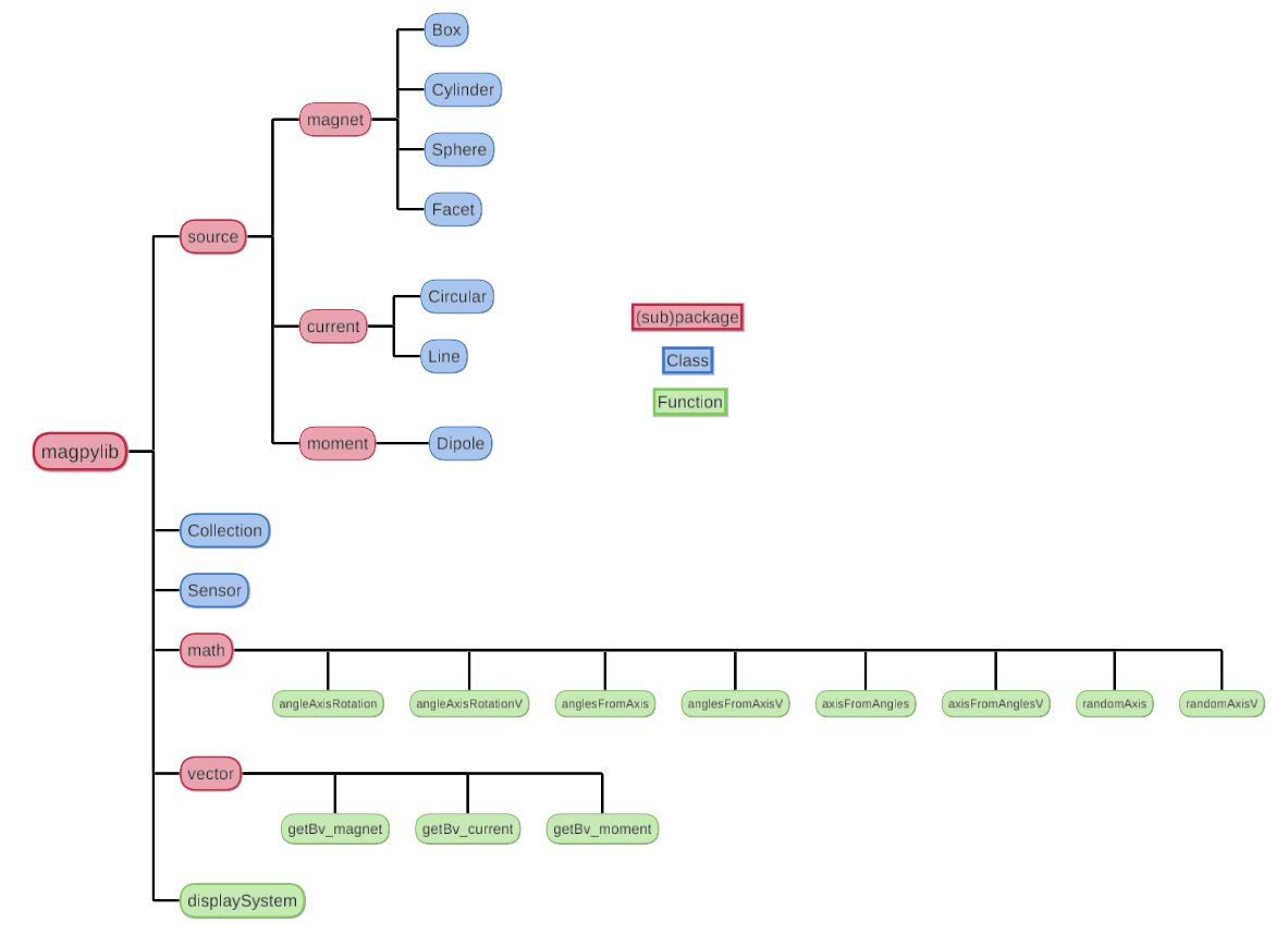
Figure: Outline of library structure.

Check out the Index and Module Index for more details.

Units and IO types¶

In magpylib all inputs and outputs are made in the physical units of

Millimeter for lengths
Degree for angles
Millitesla for magnetization/remanence, magnetic moment and magnetic field,
Ampere for currents.

Unless specifically state otherwise in the docstring (see vector package), scalar input can be of int or float type and vector/matrix input can be given either in the form of a list, as a tuple or as a numpy.array.

The library output and all object attributes are either of numpy.float64 or numpy.array64 type.

The Source Class¶

This is the core class of the library. The idea is that source objects represent physical magnetic field sources in Cartesian three-dimensional space. The following source types are currently implemented,

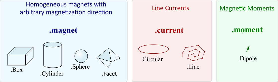
Figure: Source types currently available in magpylib.

All source objects share various attributes and methods. The attributes characterize the source (e.g. position, orientation, dimension) while the methods can be used for geometric manipulation and for calculating the magnetic field. The figure below gives a graphical overview.

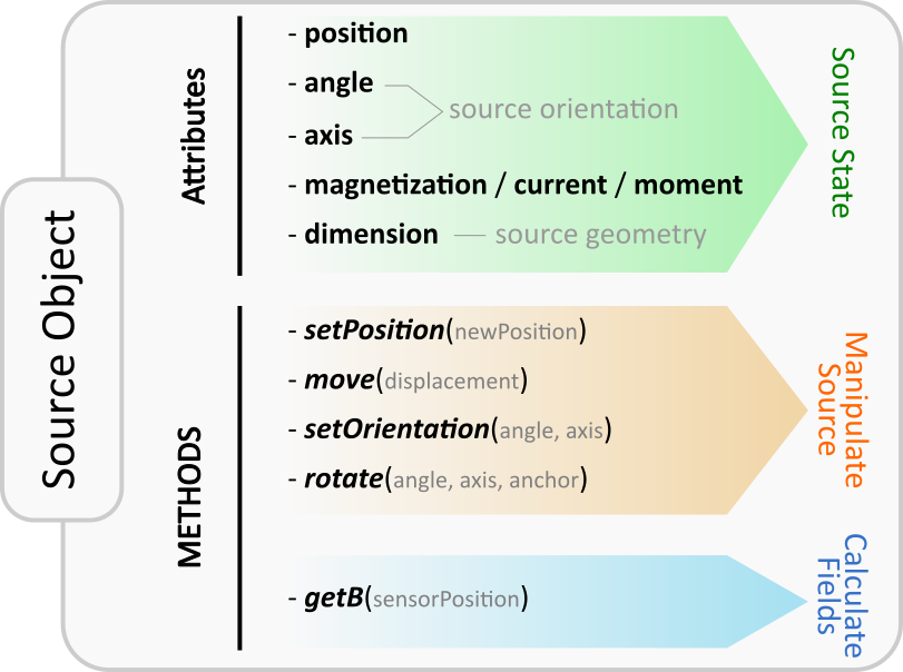
Figure: Illustration of attributes and methods of the source class objects.

Position and Orientation¶

The most fundamental properties of a source object s are position and orientation which are represented through the attributes s.position (arr3), s.angle (float) and s.axis (arr3). At source initialization, if no values are specified, the source object is initialized by default with position=(0,0,0), and init orientation defined to be angle=0 and axis=(0,0,1).

Due to their different nature each source type is characterized by different attributes. However, in general the position attribute refers to the position of the geometric center of the source. The init orientation generally defines sources standing upright oriented along the Cartesian coordinates axes, see e.g. the following image below.

An orientation of a source s given by (angle, axis ) refers to a rotation of s RELATIVE TO the init orientation about an axis specified by the s.axis vector which is anchored at s.position. The angle of this rotation is given by the s.angle attribute. Mathematically, every possible orientation can be expressed by such a single angle-axis rotation. For easier use of the angle-axis rotation and transformation to Euler angles the Math Package provides some useful methods.

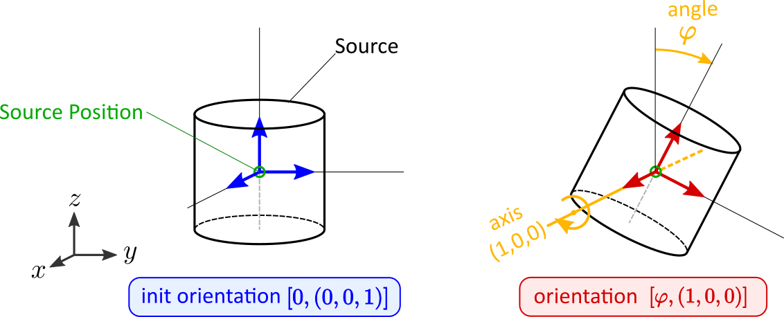
Figure: Illustration of the angle-axis system used to describe source orientations.

Dimension & Excitation¶

While position and orientation have default values, a source is defined through its geometry (e.g. cylinder) and excitation (e.g. magnetization vector) which must be initialized to provide meaning.

The dimension input specifies the size of the source. However, as each source type requires different input parameters the format is always different:

Box.dimension is a 3D array of the cuboid sides, [a,b,c]
Cylinder.dimension is a 2D array of diameter and height, [d,h]
Sphere.dimension is a float describing the diameter d
Facet.dimension is a 3x3 array of the three corner vertices, [A,B,C]
Line.dimension is a Nx3 array of N subsequent vertices, [V1,V2,V3,…]
Circular.dimension is a float describing the diameter d

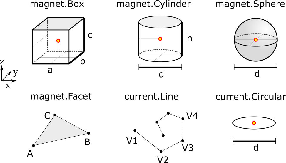
Figure: Illustration of information given by the dimension-attribute. The source positions (typically the geometric center) are indicated by the red dot.

The excitation of a source is either the magnetization, the current or the magnetic moment:

Magnet sources represent homogeneously magnetized permanent magnets (other types with radial or multipole magnetization are not implemented at this point). Such excitations are given by the magnetization (vec3) input which is always given with respect to the init orientation of the magnet.
Current sources represent electrical line currents. Their excitation is simply the electrical current in units of Ampere defined by the current (float) input.
The moment class represents a magnetic dipole moment described by the moment (vec3) input.

Detailed information about the attributes of each specific source type and how to initialize them can also be found in the respective class docstrings: Box, Cylinder, Sphere, Facet, Line, Circular, Dipole

Note

For convenience the attributes magnetization, current, dimension and position are initialized through the keywords mag, curr, dim and pos.

The following code shows how to initialize a source object, a D4H5 permanent magnet cylinder with diagonal magnetization, positioned with the center in the origin, standing upright with axis in z-direction.

from magpylib.source.magnet import Cylinder

s = Cylinder( mag = [500,0,500], # The magnetization vector in mT.
              dim = [4,5])       # dimension (diameter,height) in mm.

# no pos, angle, axis specified so default values are used

print(s.magnetization)  # Output: [500. 0. 500.]
print(s.dimension)      # Output: [4. 5.]
print(s.position)       # Output: [0. 0. 0.]
print(s.angle)          # Output: 0.0
print(s.axis)           # Output: [0. 0. 1.]

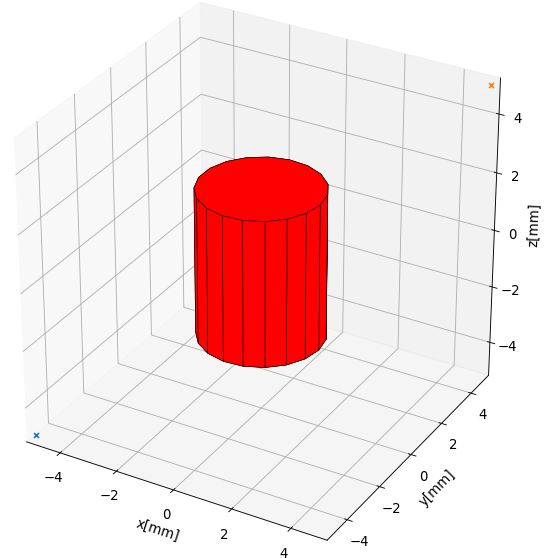
Figure: Magnet geometry created by above code: A cylinder which stands upright with geometric center at the origin.

Methods for Geometric Manipulation¶

In most cases we want to move the source to a designated position, orient it in a desired way or change its dimension dynamically. There are several ways to achieve this:

At initialization:

When initializing the source we can set all attributes as desired. So instead of moving one source around one could create a new source for each parameter set of interest.

Manipulation after initialization:

We initialize the source and manipulate it afterwards as desired by

directly setting the source attributes (e.g. s.position=newPosition),
or by using provided methods of manipulation.

The latter is often the most practical and intuitive way. To this end the source class provides a set of methods for convenient geometric manipulation. The methods include setPosition and move for translation of the objects as well as setOrientation and rotate for rotation operations. Upon application they will simply modify the source object attributes accordingly.

s.setPosition(newPos): Moves the source to the position given by the argument vector (s.position -> newPos)
s.move(displacement): Moves the source by the argument vector. (s.position -> s.position + displacement)
s.setOrientation(angle,axis): Sets a new source orientation given by the arguments. (s.angle-> angle, s.axis -> axis)
s.rotate(ang,ax,anchor=anch): Rotates the source object by the angle ang about the axis ax which passes through a position given by anch. As a result, source position and orientation attributes are modified. If no value for anchor is specified, the anchor is set to the object position, which means that the object rotates about itself.

The following videos show the application of the four methods for geometric manipulation.

The following example code shows how geometric operations are applied to source objects.

from magpylib.source.magnet import Cylinder

s = Cylinder( mag = [500,0,500], dim = [4,5])

print(s.position)       # Output: [0. 0. 0.]

s.move([1,2,3])
print(s.position)       # Output: [1. 2. 3.]

s.move([1,2,3])
print(s.position)       # Output: [2. 4. 6.]

Calculating the Magnetic Field¶

To calculate the field, magpylib uses mostly analytical expressions that can be found in the literature. References, validity and discussion of these solutions can be found in the [WIP] Physics & Computation section. In a nutshell, the fields of the dipole and the currents are exact. The analytical magnet solutions deal with homogeneous, fixed magnetizations. For hard ferromagnets with large coercive fields like Ferrite, Neodyme and SmCo the error is typically below 2%.

There are two possibilities to calculate the magnetic field of a source object s:

Using the s.getB(pos) method
Using the magpylib.vector subpackage

The first method: Each source object (or collection) s has a method s.getB(pos) which returns the magnetic field generated by s at the position pos.

from magpylib.source.magnet import Cylinder
s = Cylinder( mag = [500,0,500], dim = [4,5])
print(s.getB([4,4,4]))

# Output: [ 7.69869084 15.407166    6.40155549]

Using magpylib.vector¶

The second method: In most cases one will be interested to determine the field for a set of positions, or for different magnet positions and orientations. While this can manually be achieved by looping s.getB this is computationally inefficient. For performance computation the magpylib.vector subpackage contains the getBv functions that offer quick access to VECTORIZED CODE. A discussion of vectorization, SIMD and performance is presented in the [WIP] Physics & Computation section.

The magpylib.vector.getBv functions evaluate the field for N different sets of input parameters. These N parameter sets are provided to the getBv functions as arrays of size N for each input (e.g. an Nx3 array for the N different positions):

getBv_magnet(type, MAG, DIM, POSo, POSm, [angs1,angs2,...], [AXIS1,AXIS2,...], [ANCH1,ANCH2,...])

type is a string that specifies the magnet geometry (e.g. ‘box’ or ‘sphere’).
MAG is an Nx3 array of magnetization vectors.
DIM is an Nx3 array of magnet dimensions.
POSo is an Nx3 array of observer positions.
POSm is an Nx3 array of initial (before rotation) magnet positions.
The inputs [angs1, angs2, ...], [AXIS1, AXIS2, ...], [ANCH1, ANCH2, ...] are a lists of N/Nx3 arrays that correspond to angles, axes and anchors of rotation operations. By providing multiple list entries one can apply subsequent rotation operations. By ommitting these inputs it is assumed that no rotations are applied.

As a rule of thumb, s.getB() will be faster than getBv for ~5 or less field evaluations while the vectorized code will be up to ~100 times faster for 10 or more field evaluations. To achieve this performance it is critical that one follows the vectorized code paradigm (use only numpy native) when creating the getBv inputs. This is demonstrated in the following example where the magnetic field at a fixed observer position is calculated for a magnet that moves linearly in x-direction above the observer.

import magpylib as magpy
import numpy as np

# vector size: we calculate the field N times with different inputs
N = 1000

# Constant vectors, specify dtype
mag  = np.array([0,0,1000.])    # magnet magnetization
dim  = np.array([2,2,2.])       # magnet dimension
poso = np.array([0,0,-4.])      # position of observer

# magnet x-positions
xMag = np.linspace(-10,10,N)

# magpylib classic ---------------------------

Bc = np.zeros((N,3))
for i,x in enumerate(xMag):
    s = magpy.source.magnet.Box(mag,dim,[x,0,0])
    Bc[i] = s.getB(poso)

# magpylib vector ---------------------------

# Vectorizing input using numpy native instead of python loops
MAG = np.tile(mag,(N,1))
DIM = np.tile(dim,(N,1))
POSo = np.tile(poso,(N,1))
POSm = np.c_[xMag,np.zeros((N,2))]

# Evaluation of the N fields using vectorized code
Bv = magpy.vector.getBv_magnet('box',MAG,DIM,POSo,POSm)

# result -----------------------------------
# Bc == Bv    ... up to some 1e-16
# Copare classic and vector computation times using e.g. time.perf_counter()

More examples of vectorized code can be found in the Vectorized Code Example section.

Warning

The functions included in the magpylib.vector package do not check the input format. All input must be in the form of numpy arrays.

Collections¶

The idea behind the top level magpylib.Collection class is to group multiple source objects for common manipulation and evaluation of the fields.

In principle a collection c is simply a list of source objects that are collected in the attribute c.sources (list). Operations applied individually to the collection will be applied to all sources that are part of the collection.

Collections can be constructed at initialization by simply giving the sources objects as arguments. It is possible to add single sources, lists of multiple sources and even other collection objects. All sources are simply added to the sources attribute of the target collection.

With the collection kwarg dupWarning=True, adding multiples of the same source will be prevented, and a warning will be displayed informing the user that a source object is already in the collection’s source attribute. Adding the same object multiple times can be done by setting dupWarning=False.

In addition, the collection class features methods to add and remove sources for command line like manipulation. The method c.addSources(*sources) will add all sources given to it to the collection c. The method c.removeSource(ref) will remove the referenced source from the collection. Here the ref argument can be either a source or an integer indicating the reference position in the collection, and it defaults to the latest added source in the collection.

import magpylib as magpy

#define some magnet objects
mag1 = magpy.source.magnet.Box(mag=[1,2,3],dim=[1,2,3])
mag2 = magpy.source.magnet.Box(mag=[1,2,3],dim=[1,2,3],pos=[5,5,5])
mag3 = magpy.source.magnet.Box(mag=[1,2,3],dim=[1,2,3],pos=[-5,-5,-5])

#create/manipulate collection and print source positions
c = magpy.Collection(mag1,mag2,mag3)
print([s.position for s in c.sources])
#OUTPUT: [array([0., 0., 0.]), array([5., 5., 5.]), array([-5., -5., -5.])]

c.removeSource(1)
print([s.position for s in c.sources])
#OUTPUT: [array([0., 0., 0.]), array([-5., -5., -5.])]

c.addSources(mag2)
print([s.position for s in c.sources])
#OUTPUT: [array([0., 0., 0.]), array([-5., -5., -5.]), array([5., 5., 5.])]

All methods of geometric operation, setPosition, move, setOrientation and rotate are also methods of the collection class. A geometric operation applied to a collection is directly applied to each object within that collection individually. In practice this means that a whole group of magnets can be rotated about a common pivot point with a single command.

For calculating the magnetic field that is generated by a whole collection the method getB is also available. The total magnetic field is simply given by the superposition of the fields of all sources.

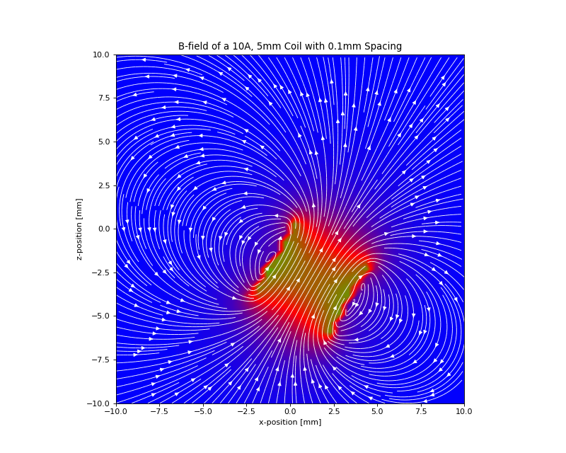
Figure: Collection Example. Circular current sources are grouped into a collection to form a coil. The whole coil is then geometrically manipulated and the total magnetic field is calculated and shown in the xz-plane.

The Sensor Class¶

The getB method will always calculate the field in the underlying canonical basis. But often one is dealing with moving and tilting sensors. For this magpylib also offers a magpylib.Sensor class.

Geometrically, a sensor object sens behaves just like a source object, having position and orientation attributes that can be set using the convenient methods sens.setPosition, sens.move, sens.setOrientation and sens.rotate.

To return the field of the source s as seen by the sensor one can use the method sens.getB(s). Here s can be a source object or a collection of sources.

import magpylib as magpy

# define sensor
sens = magpy.Sensor(pos=[5,0,0])

# define source
s = magpy.source.magnet.Sphere(mag=[123,0,0],dim=5)

# determine sensor-field
B1 = sens.getB(s)

# rotate sensor about itself (no anchor specified)
sens.rotate(90,[0,0,1])

# determine sensor-field
B2 = sens.getB(s)

# print fields
print(B1)   # output: [10.25  0.  0.]
print(B2)   # output: [0. -10.25  0.]

Display System Graphically¶

Then top level function displaySystem(c) can be used to quickly check the geometry of a source-sensor-marker assembly graphically in a 3D plot. Here c can be a source, a list of sources or a collection. displaySystem uses the matplotlib package and its limited capabilities of 3D plotting which often results in bad object overlapping.

displaySystem(c) comes with several keyword arguments:

markers=listOfPos for displaying designated reference positions. By default a marker is set at the origin. By providing [a,b,c,'text'] instead of just a simple position vector 'text' is displayed with the marker.
suppress=True for suppressing the immediate figure output when the function is called. To do so it is necessary to deactivate the interactive mode by calling pyplot.ioff(). With Spyder’s IPython Inline plotting, graphs made with displaySystem() can be blank if the suppress=True option is not used. Set IPython Graphics backend to Automatic or Qt5 instead of Inline in settings/IPython console/Graphics method to address this.
direc=True for displaying current and magnetization directions in the figure.
subplotAx=None for displaying the plot on a designated figure subplot instance.
figsize=(8,8) for setting the size of the output graphic.

The following example code shows how to use displaySystem():

import magpylib as magpy

# create sources
s1 = magpy.source.magnet.Cylinder( mag = [1,1,0],dim = [4,5], pos = [0,0,5])
s2 = magpy.source.magnet.Box( mag = [0,0,-1],dim = [1,2,3],pos=[0,0,-5])
s3 = magpy.source.current.Circular( curr = 1, dim =10)

#create collection
c = magpy.Collection(s1,s2,s3)

# create sensors
se1 = magpy.Sensor(pos=[10,0,0])
se2 = magpy.Sensor(pos=[10,0,0])
se3 = magpy.Sensor(pos=[10,0,0])
se2.rotate(70,[0,0,1],anchor=[0,0,0])
se3.rotate(140,[0,0,1],anchor=[0,0,0])

#display system
markerPos = [(0,0,0,'origin'),(10,10,10),(-10,-10,-10)]
magpy.displaySystem(c,sensors=[se1,se2,se3],markers=markerPos)

(Source code, png, hires.png, pdf)

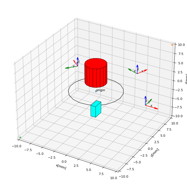
Figure: Several magnet and sensor objects are created and manipulated. Using displaySystem() they are shown in a 3D plot together with some markers which allows one to quickly check if the system geometry is ok.

Complex Magnet Geometries¶

As a result of the superposition principle complex magnet shapes and inhomogeneous magnetizations can be generated by combining multiple sources. Specifically, when two magnets overlap in this region a vector union applies. This means that in the overlap the magnetization vector is given by the sum of the two vectors of each object.

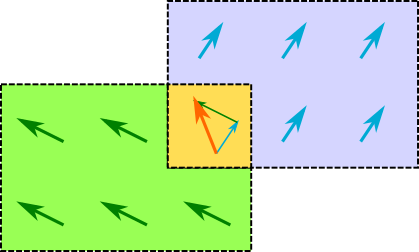
Figure: Schematic of the vector union principle for magnetizations.

Geometric addition is simply achieved by placing magnets with similar magnetization next to each other. Subtraction is realized by placing a small magnet with opposite magnetization inside a large magnet. The magnetization vectors cancel in the overlap, meaning that a small volume is cut out from a larger one. An example of a hollow cylinder is given in the examples section: Complex Magnet Shapes: Hollow Cylinder.

Math Package¶

The math package provides several practical functions that relate angle-axis (quaternion) rotations with the Euler angle rotations. All functions are also available in their vectorized versions for performance computation.

anglesFromAxis(axis): This function takes an arbitrary axis argument (vec3) and returns its orientation given by the angles (phi, theta) that are defined as in spherical coordinates. phi is the azimuth angle and theta is the polar angle.
```
import magpylib as magpy

angles = magpy.math.anglesFromAxis([1,1,0])
print(angles)

# Output = [45. 90.]
```
anglesFromAxisV(AXIS): This is the vectorized version of anglesFromAxis. It takes an Nx3 array of axis-vectors and returns an Nx2 array of angle pairs. Each angle pair is (phi,theta) which are azimuth and polar angle in a spherical coordinate system respectively.
```
import numpy as np
import magpylib as magpy

AX = np.array([[0,0,1],[0,0,1],[1,0,0]])
ANGS = magpy.math.anglesFromAxisV(AX)
print(ANGS)

# Output: [[0. 0.]  [90. 90.]  [0. 90.]])
```
axisFromAngles(angles): This function generates an axis (vec3) from the angle pair angles=(phi,theta). Here phi is the azimuth angle and theta is the polar angle of a spherical coordinate system.
```
import magpylib as magpy

ax = magpy.math.axisFromAngles([90,90])
print(ax)

# Output: [0.0  1.0  0.0]
```
axisFromAnglesV(ANGLES): This is the vectorized version of axisFromAngles. It generates an Nx3 array of axis vectors from the Nx2 array of input angle pairs angles. Each angle pair is (phi,theta) which are azimuth and polar angle in a spherical coordinate system respectively.
```
import magpylib as magpy
import numpy as np

ANGS = np.array([[0,90],[90,180],[90,0]])
AX = magpy.math.axisFromAnglesV(ANGS)
print(np.around(AX,4))

# Output: [[1.  0. 0.]  [0. 0. -1.]  [0. 0. 1.]]
```
randomAxis(): Designed for Monte Carlo simulations, this function returns a random axis (arr3) of length 1 with equal angular distribution.
```
import magpylib as magpy

ax = magpy.math.randomAxis()
print(ax)

# Output: [-0.24834468  0.96858637  0.01285925]
```

randomAxisV(N): This is the vectorized version of randomAxis. It simply returns an Nx3 array of random vectors.

import magpylib as magpy

AXS = magpy.math.randomAxisV(3)
print(AXS)

#Output: [[ 0.39480364 -0.53600779 -0.74620757]
#         [ 0.02974442  0.10916333  0.9935787 ]
#         [-0.54639126  0.76659756 -0.33731997]]

angleAxisRotation(pos, angle, axis, anchor=[0,0,0]): This function applies an angle-axis rotation. The position vector pos (vec3) is rotated by the angle angle (float) about an axis defined by the axis vector (vec3) which passes through the anchor position (vec3). The anchor argument is optional and is set to anchor=[0,0,0] if ommitted.
```
import magpylib as magpy

pos = [1,1,0]
angle = -90
axis = [0,0,1]
anchor = [1,0,0]

posNew = magpy.math.angleAxisRotation(pos,angle,axis,anchor)
print(posNew)

# Output = [2. 0. 0.]
```

angleAxisRotationV(POS, ANG, AXS, ANCH): This is the vectorized version of angleAxisRotation. Each entry of POS (arrNx3) is rotated according to the angles ANG (arrN), about the axis vectors AXS (arrNx3) which pass throught the anchors ANCH (arrNx3) where N refers to the length of the input vectors.

import magpylib as magpy
import numpy as np

POS = np.array([[1,0,0]]*5) # avoid this slow Python loop for performance conputation
ANG = np.linspace(0,180,5)
AXS = np.array([[0,0,1]]*5) # avoid this slow Python loop for performance conputation
ANCH = np.zeros((5,3))

POSnew = magpy.math.angleAxisRotationV(POS,ANG,AXS,ANCH)
print(np.around(POSnew,4))

# Output: [[ 1.      0.      0.    ]
#          [ 0.7071  0.7071  0.    ]
#          [ 0.      1.      0.    ]
#          [-0.7071  0.7071  0.    ]
#          [-1.      0.      0.    ]]