Example Codes
This section includes a few code examples that show how the library can be used and what i can be used for. A detailed technical library documentation can be found in the Documentation v2.0.1b.
Contents
Simplest Example
The simplest possible example - calculate the B-field of a cylinder with 3 lines of code.
from magpylib.source.magnet import Cylinder
s = Cylinder( mag = [0,0,350], dim = [4,5])
print(s.getB([4,4,4]))

# Output: [ 5.08641867  5.08641867 -0.60532983]
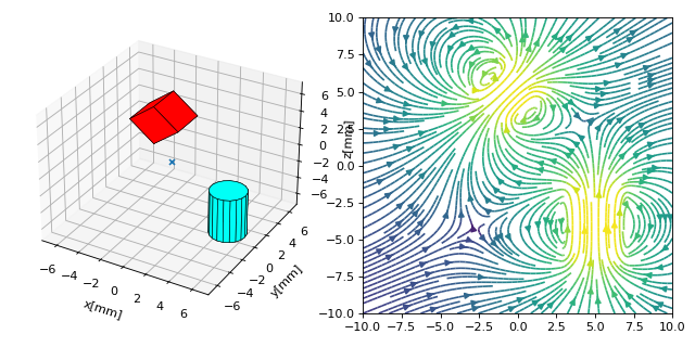
Basic Functionality: The Field of a Collection
In this example the basic functionality is outlined. Two magnet objects are created and geometrically manipulated. The system geometry is then displayed using the displaySystem function. Finally, the field is calculated on a grid and displayed in the xz-plane.
# imports
import numpy as np
import matplotlib.pyplot as plt
import magpylib as magpy

# create figure
fig = plt.figure(figsize=(8,4))
ax1 = fig.add_subplot(121, projection='3d')  # this is a 3D-plotting-axis
ax2 = fig.add_subplot(122)                   # this is a 2D-plotting-axis

# create magnets
s1 = magpy.source.magnet.Box(mag=[0,0,600],dim=[3,3,3],pos=[-4,0,3])
s2 = magpy.source.magnet.Cylinder(mag=[0,0,500], dim=[3,5])

# manipulate magnets
s1.rotate(45,[0,1,0],anchor=[0,0,0])
s2.move([5,0,-4])

# create collection
c = magpy.Collection(s1,s2)

# display system geometry on ax1
magpy.displaySystem(c,subplotAx=ax1,suppress=True)

# calculate B-field on a grid
xs = np.linspace(-10,10,29)
zs = np.linspace(-10,10,29)
Bs = np.array([[c.getB([x,0,z]) for x in xs] for z in zs])

# display field in xz-plane using matplotlib
X,Z = np.meshgrid(xs,zs)
U,V = Bs[:,:,0], Bs[:,:,2]
ax2.streamplot(X, Z, U, V, color=np.log(U**2+V**2),density=2)

plt.show()
(Source code, png, hires.png, pdf)
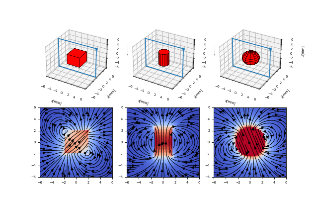
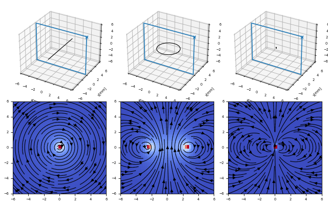
The Source Objects and their Fields
In this example we define all currently implemented source objects and display their fields. Notice that the respective magnetization vectors are chosen arbitrarily.
import magpylib as magpy
import numpy as np
from matplotlib import pyplot as plt

# set font size and define figures
plt.rcParams.update({'font.size': 6})

fig1 = plt.figure(figsize=(8, 5))
axsA = [fig1.add_subplot(2,3,i, projection='3d') for i in range(1,4)]
axsB = [fig1.add_subplot(2,3,i) for i in range(4,7)]

fig2 = plt.figure(figsize=(8, 5))
axsA += [fig2.add_subplot(2,3,i, projection='3d') for i in range(1,4)]
axsB += [fig2.add_subplot(2,3,i) for i in range(4,7)]

# position grid
ts = np.linspace(-6,6,50)
posis = np.array([(x,0,z) for z in ts for x in ts])
X,Y = np.meshgrid(ts,ts)

# create the source objects
s1 = magpy.source.magnet.Box(mag=[500,0,500], dim=[4,4,4])                #Box
s2 = magpy.source.magnet.Cylinder(mag=[0,0,500], dim=[3,5])               #Cylinder
s3 = magpy.source.magnet.Sphere(mag=[-200,0,500], dim=5)                  #Sphere
s4 = magpy.source.current.Line(curr=10, vertices=[(0,-5,0),(0,5,0)])      #Line
s5 = magpy.source.current.Circular(curr=10, dim=5)                        #Circular
s6 = magpy.source.moment.Dipole(moment=[0,0,100])                         #Dipole

for i,s in enumerate([s1,s2,s3,s4,s5,s6]):

    # display system on respective axes, use marker to zoom out
    magpy.displaySystem(s,subplotAx=axsA[i],markers=[(6,0,6)],suppress=True)
    axsA[i].plot([-6,6,6,-6,-6],[0,0,0,0,0],[-6,-6,6,6,-6])

    # plot field on respective axes
    B = np.array([s.getB(p) for p in posis]).reshape(50,50,3)
    axsB[i].pcolor(X,Y,np.linalg.norm(B,axis=2),cmap=plt.cm.get_cmap('coolwarm'))   # amplitude
    axsB[i].streamplot(X, Y, B[:,:,0], B[:,:,2], color='k',linewidth=1)             # field lines

plt.show()
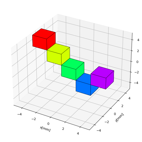
Translation, Orientation and Rotation Basics
Translation of magnets can be realized in three ways, using the methods move and setPosition, or by directly setting the object position attribute.
import numpy as np
import magpylib as magpy
from magpylib.source.magnet import Box

# fixed magnet parameters
M = [0,0,1] #magnetization
D = [2,2,2] #dimension

# Translation of magnets can be realized in several ways
s1 = Box(mag=M, dim=D, pos = [-4,0, 4])

s2 = Box(mag=M, dim=D, pos = [-2,0, 4])
s2.move([0,0,-2])

s3 = Box(mag=M, dim=D, pos = [ 0,0, 4])
s3.move([0,0,-2])
s3.move([0,0,-2])

s4 = Box(mag=M, dim=D, pos = [ 2,0, 4])
s4.setPosition([2,0,-2])

s5 = Box(mag=M, dim=D, pos = [ 4,0, 4])
s5.position = np.array([4,0,0])

#collection
c = magpy.Collection(s1,s2,s3,s4,s5)

#display collection
magpy.displaySystem(c,figsize=(6,6))
(Source code, png, hires.png, pdf)
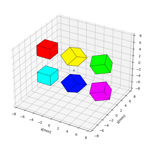
Initialize magnets with different orientations defined by classical Euler angle rotations about the three Cartesian axes. Notice that the magnetization direction is fixed with respect to the init orientation of the magnet and will rotate together with the magnet.
from magpylib.source.magnet import Box
import magpylib as magpy

# fixed magnet parameters
M = [1,0,0] #magnetization
D = [4,2,2] #dimension

# magnets with Euler angle orientations
s1 = Box(mag=M, dim=D, pos = [-4,0, 4])
s2 = Box(mag=M, dim=D, pos = [ 4,0, 4], angle=45, axis=[0,0,1])
s3 = Box(mag=M, dim=D, pos = [-4,0,-4], angle=45, axis=[0,1,0])
s4 = Box(mag=M, dim=D, pos = [ 4,0,-4], angle=45, axis=[1,0,0])

# collection
c = magpy.Collection(s1,s2,s3,s4)

# display collection
magpy.displaySystem(c,direc=True,figsize=(6,6))
(Source code, png, hires.png, pdf)
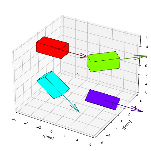
The following example shows functionality beyond Euler angle rotation. This means rotation about an arbitrary axis of choice, here (1,-1,1). The upper three boxes are initialized with different orientations. The lower three boxes are all initialized with init orientation and are then rotated (about themselves) to achieve the same result as above.
import magpylib as magpy
from magpylib.source.magnet import Box

# fixed magnet parameters
M = [0,0,1] #magnetization
D = [3,3,3] #dimension

# rotation axis
rax = [-1,1,-1]

# magnets with different orientations
s1 = Box(mag=M, dim=D, pos=[-6,0,4], angle=0, axis=rax)
s2 = Box(mag=M, dim=D, pos=[ 0,0,4], angle=45, axis=rax)
s3 = Box(mag=M, dim=D, pos=[ 6,0,4], angle=90, axis=rax)

# magnets that are rotated differently
s4 =  Box(mag=M, dim=D, pos=[-6,0,-4])
s5 =  Box(mag=M, dim=D, pos=[ 0,0,-4])
s5.rotate(45,rax)
s6 = Box(mag=M, dim=D, pos=[ 6,0,-4])
s6.rotate(90,rax)

# collect all sources
c = magpy.Collection(s1,s2,s3,s4,s5,s6)

# display collection
magpy.displaySystem(c,figsize=(6,6))
(Source code, png, hires.png, pdf)
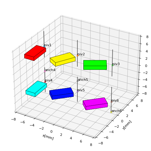
The following example shows rotations with designated anchor-axis combinations. Here we distinguish between pivot points (the closest point on the rotation axis to the magnet) and anchor points which are simply required to define an axis in 3D space (together with a direction).
import magpylib as magpy
from magpylib.source.magnet import Box
import matplotlib.pyplot as plt

# define figure
fig = plt.figure(figsize=(6,6))
ax = fig.add_subplot(1,1,1, projection='3d')

# fixed magnet parameters
M = [0,0,1] #magnetization
D = [2,4,1] #dimension

# define magnets rotated with different pivot and anchor points
piv1 = [-7,0,5]
s1 = Box(mag=M, dim=D, pos = [-7,-3,5])

piv2 = [0,0,5]
s2 = Box(mag=M, dim=D, pos = [0,-3,5])
s2.rotate(-30,[0,0,1],anchor=piv2)

piv3 = [7,0,5]
s3 = Box(mag=M, dim=D, pos = [7,-3,5])
s3.rotate(-60,[0,0,1],anchor=piv3)

piv4 = [-7,0,-5]
anch4 = [-7,0,-2]
s4 = Box(mag=M, dim=D, pos = [-7,-3,-5])

piv5 = [0,0,-5]
anch5 = [0,0,-2]
s5 = Box(mag=M, dim=D, pos = [0,-3,-5])
s5.rotate(-45,[0,0,1],anchor=anch5)

piv6 = [7,0,-5]
anch6 = [7,0,-8]
s6 = Box(mag=M, dim=D, pos = [7,-3,-5])
s6.rotate(-45,[0,0,1],anchor=anch6)

# collect all sources
c = magpy.Collection(s1,s2,s3,s4,s5,s6)

# draw rotation axes
for x in [-7,0,7]:
    for z in [-5,5]:
        ax.plot([x,x],[0,0],[z-3,z+4],color='.3')

# define markers
Ms = [piv1+['piv1'], piv2+['piv2'], piv3+['piv3'], piv4+['piv4'],
      piv5+['piv5'], piv6+['piv6'], anch4+['anch4'],anch5+['anch5'],anch6+['anch6']]

# display system
magpy.displaySystem(c,subplotAx=ax,markers=Ms,suppress=True)

plt.show()
(Source code, png, hires.png, pdf)
Collections can be manipulated using the previous logic as well. Notice how objects can be grouped into collections and sub-collections for common manipulation. For rotations keep in mind that if an anchor is not provided, all objects will rotate relative to their own center.
import magpylib as magpy
from magpylib.source.current import Circular
from numpy import linspace

# windings of three parts of a coil
coil1a = [Circular(curr=1,dim=3,pos=[0,0,z]) for z in linspace( -3,-1,10)]
coil1b = [Circular(curr=1,dim=3,pos=[0,0,z]) for z in linspace( -1, 1,10)]
coil1c = [Circular(curr=1,dim=3,pos=[0,0,z]) for z in linspace(  1, 3,10)]

# create collection and manipulate step by step
c1 = magpy.Collection(coil1a)
c1.move([-1,-1,0])
c1.addSources(coil1b)
c1.move([-1,-1,0])
c1.addSources(coil1c)
c1.move([-1,-1,0])

# windings of three parts of another coil
coil2a = [Circular(curr=1,dim=3,pos=[3,3,z]) for z in linspace(-3,-1,15)]
coil2b = [Circular(curr=1,dim=3,pos=[3,3,z]) for z in linspace( -1,1,15)]
coil2c = [Circular(curr=1,dim=3,pos=[3,3,z]) for z in linspace( 1,3,15)]

# create individual sub-collections
c2a = magpy.Collection(coil2a)
c2b = magpy.Collection(coil2b)
c2c = magpy.Collection(coil2c)

# combine sub-collections to one big collection
c2 = magpy.Collection(c2a,c2b,c2c)

# still manipulate each individual sub-collection
c2a.rotate(-15,[1,-1,0],anchor=[0,0,0])
c2c.rotate(15,[1,-1,0],anchor=[0,0,0])

# combine all collections and display system
c3 = magpy.Collection(c1,c2)
magpy.displaySystem(c3,figsize=(6,6))
(Source code, png, hires.png, pdf)
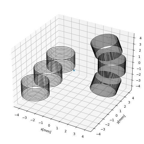
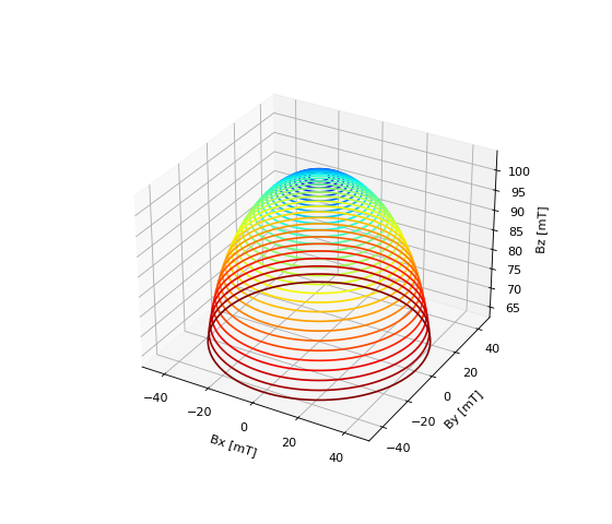
Magnet Motion: Simulating a Magnetic Joystick
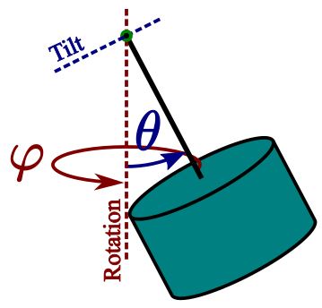
In this example a joystick is simulated. A magnetic joystick is realized by a rod that can tilt freely (two degrees of freedom) about a center of tilt. The upper part of the rod is the joystick handle. At the bottom of the rod a cylindrical magnet (dim=(D,H)) with axial magnetization `mag=[0,0,M0] is fixed. The magnet lies at a distance d below the center of tilt. The system is constructed such that, when the joystick is in the center position a sensor lies at distance gap below the magnet and in the origin of a Cartesian coordinate system. The magnet thus moves with the joystick above the fixed sensor.
In the following program the magnetic field is calculated for all degrees of freedom. Different tilt angles are set by rotation about the center of tilt by the angle th (different colors). Then the tilt direction is varied from 0 to 360 degrees by simulating the magnet motion as rotation about the z-axis, see also the following sketch.
from magpylib.source.magnet import Cylinder
import matplotlib.pyplot as plt
import numpy as np

# system parameters
D,H = 5,4       #magnet dimension
M0 = 1200       #magnet magnetization amplitude
gap = 3         #airgap
d = 5           #distance magnet to center of tilt
thMAX = 15      #maximal joystick tilt angle

# define figure
fig = plt.figure(figsize=(7,6))
ax = plt.axes(projection='3d')
cm = plt.get_cmap("jet") #colormap

# set tilt angle
for th in np.linspace(1,thMAX,30):

    # store fields here
    Bs = np.zeros([181,3])

    # create magnet for joystick in center position
    s = Cylinder(dim=[D,H],mag=[0,0,M0],pos=[0,0,H/2+gap])

    # set joystick tilt th
    s.rotate(th,[0,1,0],anchor=[0,0,gap+H+d])

    # rotate joystick for fixed tilt
    for i in range(181):

        # calculate field (sensor at [0,0,0]) and store in Bs
        Bs[i] = s.getB([0,0,0])

        # rotate magnet to next position
        s.rotate(2,[0,0,1],anchor=[0,0,0])

    # plot fields
    ax.plot(Bs[:,0],Bs[:,1],Bs[:,2],color=cm(th/15))

# annotate
ax.set(
       xlabel = 'Bx [mT]',
       ylabel = 'By [mT]',
       zlabel = 'Bz [mT]')

# display
plt.show()
(Source code, png, hires.png, pdf)
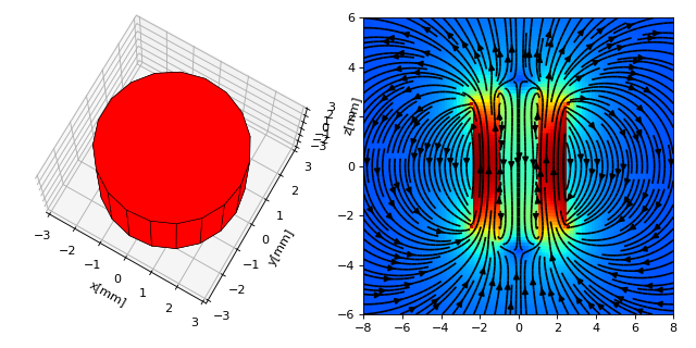
Complex Magnet Shapes: Hollow Cylinder
The superposition principle allows us to calculate complex magnet shapes by addition and subtraction operations. An example application for this is the field of an axially magnetized hollow cylinder. The hollow part is cut out from the outer cylinder by placing a second, smaller cylinder inside with opposite magnetization. Unfortunately the displaySystem method cannot properly display such objects intersecting with each other.
import numpy as np
import matplotlib.pyplot as plt
from magpylib.source.magnet import Cylinder
import magpylib as magpy

# create collection of two magnets
s1 = Cylinder(mag=[0,0,1000], dim=[5,5])
s2 = Cylinder(mag=[0,0,-1000], dim=[2,6])
c = magpy.Collection(s1,s2)

# create positions
xs = np.linspace(-8,8,100)
zs = np.linspace(-6,6,100)
posis = [[x,0,z] for z in zs for x in xs]

# calculate field and amplitude
B = [c.getB(pos) for pos in posis]
Bs = np.array(B).reshape([100,100,3]) #reshape
Bamp = np.linalg.norm(Bs,axis=2)

# define figure with a 2d and a 3d axis
fig = plt.figure(figsize=(8,4))
ax1 = fig.add_subplot(121,projection='3d')
ax2 = fig.add_subplot(122)

# add displaySystem on ax1
magpy.displaySystem(c,subplotAx=ax1,suppress=True)
ax1.view_init(elev=75)

# amplitude plot on ax2
X,Z = np.meshgrid(xs,zs)
ax2.pcolor(xs,zs,Bamp,cmap='jet',vmin=-200)

# plot field lines on ax2
U,V = Bs[:,:,0], Bs[:,:,2]
ax2.streamplot(X,Z,U,V,color='k',density=2)

#display
plt.show()
(Source code, png, hires.png, pdf)
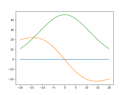
Vectorized Code Example
In this example a magnet is tilted above a sensor just like in a 1D-joystick system. The magnetic field is computed using vectorized code, taking care to create the getBv input using numpy native methods only.
import magpylib as magpy
import numpy as np
import matplotlib.pyplot as plt

import time

# vector size: we calculate the field N times with different inputs
N = 100000

# Constant vectors
mag  = np.array([0,0,1000])    # magnet magnetization
dim  = np.array([2,2,2])       # magnet dimension
poso = np.array([0,0,0])       # position of observer
posm = np.array([0,0,3])       # initial magnet position
anch = np.array([0,0,8])       # rotation anchor
axis = np.array([1,0,0])       # rotation axis

# different angles for each evaluation
angs = np.linspace(-20,20,N)

# Vectorizing input using numpy native instead of python loops
MAG = np.tile(mag,(N,1))
DIM = np.tile(dim,(N,1))
POSo = np.tile(poso,(N,1))
POSm = np.tile(posm,(N,1))  # inital magnet positions before rotations are applied
ANCH = np.tile(anch,(N,1))  # always same axis
AXIS = np.tile(axis,(N,1))  # always same anchor

# N-times evalulation of the field with different inputs
Bv = magpy.vector.getBv_magnet('box',MAG,DIM,POSo,POSm,[angs],[AXIS],[ANCH])

# plot field
plt.plot(angs,Bv[:,0])
plt.plot(angs,Bv[:,1])
plt.plot(angs,Bv[:,2])

plt.show()
(Source code, png, hires.png, pdf)