Physics & Computation¶

The analytical solutions¶

Permanent Magnets

Magnetic field computations in Magpylib are based on known analytical solutions (formulas) to permanent magnet and current problems. For Magpylib we have used the following references:

Field of cuboid magnets: [1999Yang, 2005Engel-Herbert, 2013Camacho]
Field of cylindrical magnets: [1994Furlani, 2009Derby]
Field of facet bodies: [2009Janssen, 2013Rubeck]
Field of circular line current: [1950Smythe, 2001Simpson, 2017Ortner]
all others derived by hand

A short reflection on how these formulas can be achieved: In magnetostatics (no currents) the magnetic field becomes conservative (Maxwell: $\nabla \times {\bf H} = 0$ ) and can thus be expressed through the magnetic scalar potential $\Phi_m$ :

${\bf H} = -\nabla\cdot\Phi_m$

The solution to this equation can be expressed by an integral over the magnetization distribution ${\bf M}({\bf r})$ as

$\Phi_m({\bf r}) = \frac{1}{4\pi}\int_{V'}\frac{\nabla'\cdot {\bf M}({\bf r}')}{|{\bf r}-{\bf r}'|}dV'+\frac{1}{4\pi}\oint_{S'}\frac{{\bf n}'\cdot {\bf M}({\bf r}')}{|{\bf r}-{\bf r}'|}dS'$

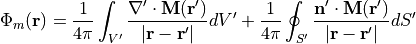
where ${\bf r}$ denotes the position, $V$ is the magnetized volume with surface $S$ and normal vector ${\bf n}$ onto the surface. This solution is derived in detail e.g. in [1999Jackson].

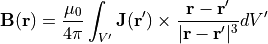
Currents

The fields of currents are directly derived using the law of Biot-Savart with the current distribution ${\bf J}({\bf r})$ :

${\bf B}({\bf r}) = \frac{\mu_0}{4\pi}\int_{V'} {\bf J}({\bf r}')\times \frac{{\bf r}-{\bf r}'}{|{\bf r}-{\bf r}'|^3} dV'$

In some special cases (simple shapes, homogeneous magnetizations and current distributions) the above integrals can be worked out directly to give analytical formulas (or simple, fast converging series). The derivations can be found in the respective references. A noteworthy comparison between the Coulombian approach and the Amperian current model is given in [2009Ravaud].

References

[1999Yang] Z. J. Yang et al., “Potential and force between a magnet and a bulk Y1Ba2Cu3O7-d superconductor studied by a mechanical pendulum”, Superconductor Science and Technology 3(12):591, 1999
[2005 Engel-Herbert] R. Engel-Herbert et al., Journal of Applied Physics 97(7):074504 - 074504-4 (2005)
[2013 Camacho] J.M. Camacho and V. Sosa, “Alternative method to calculate the magnetic field of permanent magnets with azimuthal symmetry”, Revista Mexicana de Fisica E 59 8–17, 2013
[1994Furlani] E. P. Furlani, S. Reanik and W. Janson, “A Three-Dimensional Field Solution for Bipolar Cylinders”, IEEE Transaction on Magnetics, VOL. 30, NO. 5, 1994
[2009Derby] N. Derby, “Cylindrical Magnets and Ideal Solenoids”, arXiv:0909.3880v1, 2009
[1950Smythe] W.B. Smythe, “Static and dynamic electricity” McGraw-Hill New York, 1950, vol. 3.
[2001Simpson] J. Simplson et al., “Simple analytic expressions for the magnetic field of a circular current loop,” 2001.
[2017Ortner] M. Ortner et al., “Feedback of Eddy Currents in Layered Materials for Magnetic Speed Sensing”, IEEE Transactions on Magnetics ( Volume: 53, Issue: 8, Aug. 2017)
[2009Janssen] J.L.G. Janssen, J.J.H. Paulides and E.A. Lomonova, “3D ANALYTICAL FIELD CALCULATION USING TRIANGULAR MAGNET SEGMENTS APPLIED TO A SKEWED LINEAR PERMANENT MAGNET ACTUATOR”, ISEF 2009 - XIV International Symposium on Electromagnetic Fields in Mechatronics, Electrical and Electronic Engineering Arras, France, September 10-12, 2009
[2013Rubeck] C. Rubeck et al., “Analytical Calculation of Magnet Systems: Magnetic Field Created by Charged Triangles and Polyhedra”, IEEE Transactions on Magnetics, VOL. 49, NO. 1, 2013
[1999Jackson] J. D. Jackson, “Classical Electrodynamics”, 1999 Wiley, New York
[2009Ravaud] R. Ravaud and G. Lamarquand, “Comparison of the coulombian and amperian current models for calculating the magnetic field produced by radially magnetized arc-shaped permanent magnets”, HAL Id: hal-00412346

Accuracy of the Solutions and Demagnetization¶

Line currents:

The magnetic field of a wire carrying a homogeneous current density is similar (ON THE OUTSIDE ONLY) to the field of a line current in the center of the wire, which carries the total current of the wire. Current distributions become inhomogeneous at bends of the wire or when eddy currents (finite frequencies) are involved.

Magnets and Demagnetization

The anayltical solutions are exact when bodies have a homogeneous magnetization. However, real materials always have a material response which results in an inhomogeneous magnetization even when the initial magnetization is perfectly homogeneous. There is a lot of literature on such demagnetization effects.

Modern high grade permanent magnets (NdFeB, SmCo, Ferrite) have a very weak material responses (local slope of the magnetization curve, remanent permeability) of the order of $\mu_r \approx 1.05$ . In this case the analyical solutions provide an excellent approximation with less than 1% error even at close distance from the magnet surface. A detailed error analysis and discussion is presented in the appendix of [2020Malago].

Soft-Magnetic Materials

Soft-magnetic materials like iron or steel with large permeabilities $\mu_r \sim 1000$ can in principle not be modeled with Magpylib. However, when the body is static, when there is no strong local interaction with an adjacent magnet and when the body is mostly conformal one can approximate the field using the Magpylib solutions and some empirical magnetization that depends on the shape of the body, the material response and the strength of the magnetizing field.

An example would be the magnetization of a soft-magnetic metal piece in the earth magnetic field. However, even in such a case it is probably more efficient to use a simple dipole approximation.

Convergence of the diametral Cylinder solution

The diametral Cylinder solution is based on a convering series. 50 iterations are probaby ok and also set as standard. If you want to be precise increase iterations and observer the convergence behavior. Change the setting to x with

magpylib.Config.ITER_CYLINDER = x

References

[2020Malago] P. Malagò et al., Magnetic Position System Design Method Applied to Three-Axis Joystick Motion Tracking. Sensors, 2020, 20. Jg., Nr. 23, S. 6873.

Computation¶

Magpylib code is fully vectorized, written almost completly in numpy native. Magpylib automatically vectorizes the computation with complex inputs (many sources, many observers, paths) and never falls back on using loops.

Note

Maximal performance is achieved when .getB(sources, observers) is called only a single time in your program. Try not to use loops.

Of course the objective oriented interface (sensors and sources) comes with an overhead. If you want to achieve maximal performance this overhead can be avoided through direct access to the vectorized field functions with the top level function magpylib.getBv.